{% raw %}
Title: Create a Markdown Blog Post Integrating Research Details and a Featured Paper
====================================================================================
This task involves generating a Markdown file (ready for a GitHub-served Jekyll site) that integrates our research details with a featured research paper. The output must follow the exact format and conventions described below.
====================================================================================
Output Format (Markdown):
------------------------------------------------------------------------------------
---
layout: post
title: "Alleviating the Hubble tension with Torsion Condensation (TorC)"
date: 2025-07-12
categories: papers
---


 Content generated by [gemini-2.5-pro](https://deepmind.google/technologies/gemini/) using [this prompt](/prompts/content/2025-07-12-2507.09228.txt).
Image generated by [imagen-3.0-generate-002](https://deepmind.google/technologies/gemini/) using [this prompt](/prompts/images/2025-07-12-2507.09228.txt).
------------------------------------------------------------------------------------
====================================================================================
Please adhere strictly to the following instructions:
====================================================================================
Section 1: Content Creation Instructions
====================================================================================
1. **Generate the Page Body:**
- Write a well-composed, engaging narrative that is suitable for a scholarly audience interested in advanced AI and astrophysics.
- Ensure the narrative is original and reflective of the tone and style and content in the "Homepage Content" block (provided below), but do not reuse its content.
- Use bullet points, subheadings, or other formatting to enhance readability.
2. **Highlight Key Research Details:**
- Emphasize the contributions and impact of the paper, focusing on its methodology, significance, and context within current research.
- Specifically highlight the lead author ({'name': 'Sinah Legner'}). When referencing any author, use Markdown links from the Author Information block (choose academic or GitHub links over social media).
3. **Integrate Data from Multiple Sources:**
- Seamlessly weave information from the following:
- **Paper Metadata (YAML):** Essential details including the title and authors.
- **Paper Source (TeX):** Technical content from the paper.
- **Bibliographic Information (bbl):** Extract bibliographic references.
- **Author Information (YAML):** Profile details for constructing Markdown links.
- Merge insights from the Paper Metadata, TeX source, Bibliographic Information, and Author Information blocks into a coherent narrative—do not treat these as separate or isolated pieces.
- Insert the generated narrative between the HTML comments:
and
4. **Generate Bibliographic References:**
- Review the Bibliographic Information block carefully.
- For each reference that includes a DOI or arXiv identifier:
- For DOIs, generate a link formatted as:
[10.1234/xyz](https://doi.org/10.1234/xyz)
- For arXiv entries, generate a link formatted as:
[2103.12345](https://arxiv.org/abs/2103.12345)
- **Important:** Do not use any LaTeX citation commands (e.g., `\cite{...}`). Every reference must be rendered directly as a Markdown link. For example, instead of `\cite{mycitation}`, output `[mycitation](https://doi.org/mycitation)`
- **Incorrect:** `\cite{10.1234/xyz}`
- **Correct:** `[10.1234/xyz](https://doi.org/10.1234/xyz)`
- Ensure that at least three (3) of the most relevant references are naturally integrated into the narrative.
- Ensure that the link to the Featured paper [2507.09228](https://arxiv.org/abs/2507.09228) is included in the first sentence.
5. **Final Formatting Requirements:**
- The output must be plain Markdown; do not wrap it in Markdown code fences.
- Preserve the YAML front matter exactly as provided.
====================================================================================
Section 2: Provided Data for Integration
====================================================================================
1. **Homepage Content (Tone and Style Reference):**
```markdown
---
layout: home
---

The Handley Research Group stands at the forefront of cosmological exploration, pioneering novel approaches that fuse fundamental physics with the transformative power of artificial intelligence. We are a dynamic team of researchers, including PhD students, postdoctoral fellows, and project students, based at the University of Cambridge. Our mission is to unravel the mysteries of the Universe, from its earliest moments to its present-day structure and ultimate fate. We tackle fundamental questions in cosmology and astrophysics, with a particular focus on leveraging advanced Bayesian statistical methods and AI to push the frontiers of scientific discovery. Our research spans a wide array of topics, including the [primordial Universe](https://arxiv.org/abs/1907.08524), [inflation](https://arxiv.org/abs/1807.06211), the nature of [dark energy](https://arxiv.org/abs/2503.08658) and [dark matter](https://arxiv.org/abs/2405.17548), [21-cm cosmology](https://arxiv.org/abs/2210.07409), the [Cosmic Microwave Background (CMB)](https://arxiv.org/abs/1807.06209), and [gravitational wave astrophysics](https://arxiv.org/abs/2411.17663).
### Our Research Approach: Innovation at the Intersection of Physics and AI
At The Handley Research Group, we develop and apply cutting-edge computational techniques to analyze complex astronomical datasets. Our work is characterized by a deep commitment to principled [Bayesian inference](https://arxiv.org/abs/2205.15570) and the innovative application of [artificial intelligence (AI) and machine learning (ML)](https://arxiv.org/abs/2504.10230).
**Key Research Themes:**
* **Cosmology:** We investigate the early Universe, including [quantum initial conditions for inflation](https://arxiv.org/abs/2002.07042) and the generation of [primordial power spectra](https://arxiv.org/abs/2112.07547). We explore the enigmatic nature of [dark energy, using methods like non-parametric reconstructions](https://arxiv.org/abs/2503.08658), and search for new insights into [dark matter](https://arxiv.org/abs/2405.17548). A significant portion of our efforts is dedicated to [21-cm cosmology](https://arxiv.org/abs/2104.04336), aiming to detect faint signals from the Cosmic Dawn and the Epoch of Reionization.
* **Gravitational Wave Astrophysics:** We develop methods for [analyzing gravitational wave signals](https://arxiv.org/abs/2411.17663), extracting information about extreme astrophysical events and fundamental physics.
* **Bayesian Methods & AI for Physical Sciences:** A core component of our research is the development of novel statistical and AI-driven methodologies. This includes advancing [nested sampling techniques](https://arxiv.org/abs/1506.00171) (e.g., [PolyChord](https://arxiv.org/abs/1506.00171), [dynamic nested sampling](https://arxiv.org/abs/1704.03459), and [accelerated nested sampling with $\beta$-flows](https://arxiv.org/abs/2411.17663)), creating powerful [simulation-based inference (SBI) frameworks](https://arxiv.org/abs/2504.10230), and employing [machine learning for tasks such as radiometer calibration](https://arxiv.org/abs/2504.16791), [cosmological emulation](https://arxiv.org/abs/2503.13263), and [mitigating radio frequency interference](https://arxiv.org/abs/2211.15448). We also explore the potential of [foundation models for scientific discovery](https://arxiv.org/abs/2401.00096).
**Technical Contributions:**
Our group has a strong track record of developing widely-used scientific software. Notable examples include:
* [**PolyChord**](https://arxiv.org/abs/1506.00171): A next-generation nested sampling algorithm for Bayesian computation.
* [**anesthetic**](https://arxiv.org/abs/1905.04768): A Python package for processing and visualizing nested sampling runs.
* [**GLOBALEMU**](https://arxiv.org/abs/2104.04336): An emulator for the sky-averaged 21-cm signal.
* [**maxsmooth**](https://arxiv.org/abs/2007.14970): A tool for rapid maximally smooth function fitting.
* [**margarine**](https://arxiv.org/abs/2205.12841): For marginal Bayesian statistics using normalizing flows and KDEs.
* [**fgivenx**](https://arxiv.org/abs/1908.01711): A package for functional posterior plotting.
* [**nestcheck**](https://arxiv.org/abs/1804.06406): Diagnostic tests for nested sampling calculations.
### Impact and Discoveries
Our research has led to significant advancements in cosmological data analysis and yielded new insights into the Universe. Key achievements include:
* Pioneering the development and application of advanced Bayesian inference tools, such as [PolyChord](https://arxiv.org/abs/1506.00171), which has become a cornerstone for cosmological parameter estimation and model comparison globally.
* Making significant contributions to the analysis of major cosmological datasets, including the [Planck mission](https://arxiv.org/abs/1807.06209), providing some of the tightest constraints on cosmological parameters and models of [inflation](https://arxiv.org/abs/1807.06211).
* Developing novel AI-driven approaches for astrophysical challenges, such as using [machine learning for radiometer calibration in 21-cm experiments](https://arxiv.org/abs/2504.16791) and [simulation-based inference for extracting cosmological information from galaxy clusters](https://arxiv.org/abs/2504.10230).
* Probing the nature of dark energy through innovative [non-parametric reconstructions of its equation of state](https://arxiv.org/abs/2503.08658) from combined datasets.
* Advancing our understanding of the early Universe through detailed studies of [21-cm signals from the Cosmic Dawn and Epoch of Reionization](https://arxiv.org/abs/2301.03298), including the development of sophisticated foreground modelling techniques and emulators like [GLOBALEMU](https://arxiv.org/abs/2104.04336).
* Developing new statistical methods for quantifying tensions between cosmological datasets ([Quantifying tensions in cosmological parameters: Interpreting the DES evidence ratio](https://arxiv.org/abs/1902.04029)) and for robust Bayesian model selection ([Bayesian model selection without evidences: application to the dark energy equation-of-state](https://arxiv.org/abs/1506.09024)).
* Exploring fundamental physics questions such as potential [parity violation in the Large-Scale Structure using machine learning](https://arxiv.org/abs/2410.16030).
### Charting the Future: AI-Powered Cosmological Discovery
The Handley Research Group is poised to lead a new era of cosmological analysis, driven by the explosive growth in data from next-generation observatories and transformative advances in artificial intelligence. Our future ambitions are centred on harnessing these capabilities to address the most pressing questions in fundamental physics.
**Strategic Research Pillars:**
* **Next-Generation Simulation-Based Inference (SBI):** We are developing advanced SBI frameworks to move beyond traditional likelihood-based analyses. This involves creating sophisticated codes for simulating [Cosmic Microwave Background (CMB)](https://arxiv.org/abs/1908.00906) and [Baryon Acoustic Oscillation (BAO)](https://arxiv.org/abs/1607.00270) datasets from surveys like DESI and 4MOST, incorporating realistic astrophysical effects and systematic uncertainties. Our AI initiatives in this area focus on developing and implementing cutting-edge SBI algorithms, particularly [neural ratio estimation (NRE) methods](https://arxiv.org/abs/2407.15478), to enable robust and scalable inference from these complex simulations.
* **Probing Fundamental Physics:** Our enhanced analytical toolkit will be deployed to test the standard cosmological model ($\Lambda$CDM) with unprecedented precision and to explore [extensions to Einstein's General Relativity](https://arxiv.org/abs/2006.03581). We aim to constrain a wide range of theoretical models, from modified gravity to the nature of [dark matter](https://arxiv.org/abs/2106.02056) and [dark energy](https://arxiv.org/abs/1701.08165). This includes leveraging data from upcoming [gravitational wave observatories](https://arxiv.org/abs/1803.10210) like LISA, alongside CMB and large-scale structure surveys from facilities such as Euclid and JWST.
* **Synergies with Particle Physics:** We will continue to strengthen the connection between cosmology and particle physics by expanding the [GAMBIT framework](https://arxiv.org/abs/2009.03286) to interface with our new SBI tools. This will facilitate joint analyses of cosmological and particle physics data, providing a holistic approach to understanding the Universe's fundamental constituents.
* **AI-Driven Theoretical Exploration:** We are pioneering the use of AI, including [large language models and symbolic computation](https://arxiv.org/abs/2401.00096), to automate and accelerate the process of theoretical model building and testing. This innovative approach will allow us to explore a broader landscape of physical theories and derive new constraints from diverse astrophysical datasets, such as those from GAIA.
Our overarching goal is to remain at the forefront of scientific discovery by integrating the latest AI advancements into every stage of our research, from theoretical modeling to data analysis and interpretation. We are excited by the prospect of using these powerful new tools to unlock the secrets of the cosmos.
Content generated by [gemini-2.5-pro-preview-05-06](https://deepmind.google/technologies/gemini/) using [this prompt](/prompts/content/index.txt).
Image generated by [imagen-3.0-generate-002](https://deepmind.google/technologies/gemini/) using [this prompt](/prompts/images/index.txt).
```
2. **Paper Metadata:**
```yaml
!!python/object/new:feedparser.util.FeedParserDict
dictitems:
id: http://arxiv.org/abs/2507.09228v3
guidislink: true
link: http://arxiv.org/abs/2507.09228v3
updated: '2025-07-30T12:52:43Z'
updated_parsed: !!python/object/apply:time.struct_time
- !!python/tuple
- 2025
- 7
- 30
- 12
- 52
- 43
- 2
- 211
- 0
- tm_zone: null
tm_gmtoff: null
published: '2025-07-12T09:56:02Z'
published_parsed: !!python/object/apply:time.struct_time
- !!python/tuple
- 2025
- 7
- 12
- 9
- 56
- 2
- 5
- 193
- 0
- tm_zone: null
tm_gmtoff: null
title: Alleviating the Hubble tension with Torsion Condensation (TorC)
title_detail: !!python/object/new:feedparser.util.FeedParserDict
dictitems:
type: text/plain
language: null
base: ''
value: Alleviating the Hubble tension with Torsion Condensation (TorC)
summary: 'Constraints on the cosmological parameters of Torsion Condensation (TorC)
are
investigated using Planck 2018 Cosmic Microwave Background data. TorC is a case
of Poincar\''e gauge theory -- a formulation of gravity motivated by the gauge
field theories underlying fundamental forces in the standard model of particle
physics. Unlike general relativity, TorC incorporates intrinsic torsion degrees
of freedom while maintaining second-order field equations. At specific
parameter values, it reduces to the $\Lambda$CDM model, providing a natural
extension to standard cosmology. The base model of TorC introduces two
parameters beyond those in $\Lambda$CDM: the initial value of the torsion
scalar field and its time derivative -- one can absorb the latter by allowing
the dark energy density to float. To constrain these parameters, `PolyChord`
nested sampling algorithm is employed, interfaced via `Cobaya` with a modified
version of `CAMB`. Our results indicate that TorC allows for a larger inferred
Hubble constant, offering a potential resolution to the Hubble tension. Tension
analysis using the $R$-statistic shows that TorC alleviates the statistical
tension between the Planck 2018 and SH0Es 2020 datasets, though this
improvement is not sufficient to decisively favour TorC over $\Lambda$CDM in a
Bayesian model comparison. This study highlights TorC as a compelling theory of
gravity, demonstrating its potential to address cosmological tensions and
motivating further investigations of extended theories of gravity within a
cosmological context. As current and upcoming surveys -- including Euclid,
Roman Space Telescope, Vera C. Rubin Observatory, LISA, and Simons Observatory
-- deliver data on gravity across all scales, they will offer critical tests of
gravity models like TorC, making the present a pivotal moment for exploring
extended theories of gravity.'
summary_detail: !!python/object/new:feedparser.util.FeedParserDict
dictitems:
type: text/plain
language: null
base: ''
value: 'Constraints on the cosmological parameters of Torsion Condensation (TorC)
are
investigated using Planck 2018 Cosmic Microwave Background data. TorC is a
case
of Poincar\''e gauge theory -- a formulation of gravity motivated by the gauge
field theories underlying fundamental forces in the standard model of particle
physics. Unlike general relativity, TorC incorporates intrinsic torsion degrees
of freedom while maintaining second-order field equations. At specific
parameter values, it reduces to the $\Lambda$CDM model, providing a natural
extension to standard cosmology. The base model of TorC introduces two
parameters beyond those in $\Lambda$CDM: the initial value of the torsion
scalar field and its time derivative -- one can absorb the latter by allowing
the dark energy density to float. To constrain these parameters, `PolyChord`
nested sampling algorithm is employed, interfaced via `Cobaya` with a modified
version of `CAMB`. Our results indicate that TorC allows for a larger inferred
Hubble constant, offering a potential resolution to the Hubble tension. Tension
analysis using the $R$-statistic shows that TorC alleviates the statistical
tension between the Planck 2018 and SH0Es 2020 datasets, though this
improvement is not sufficient to decisively favour TorC over $\Lambda$CDM
in a
Bayesian model comparison. This study highlights TorC as a compelling theory
of
gravity, demonstrating its potential to address cosmological tensions and
motivating further investigations of extended theories of gravity within a
cosmological context. As current and upcoming surveys -- including Euclid,
Roman Space Telescope, Vera C. Rubin Observatory, LISA, and Simons Observatory
-- deliver data on gravity across all scales, they will offer critical tests
of
gravity models like TorC, making the present a pivotal moment for exploring
extended theories of gravity.'
authors:
- !!python/object/new:feedparser.util.FeedParserDict
dictitems:
name: Sinah Legner
- !!python/object/new:feedparser.util.FeedParserDict
dictitems:
name: Will Handley
- !!python/object/new:feedparser.util.FeedParserDict
dictitems:
name: Will Barker
author_detail: !!python/object/new:feedparser.util.FeedParserDict
dictitems:
name: Will Barker
author: Will Barker
arxiv_comment: "21 pages (main text: 12 pages), 9 figures, 7 tables, comments\n\
\ welcome!"
links:
- !!python/object/new:feedparser.util.FeedParserDict
dictitems:
href: http://arxiv.org/abs/2507.09228v3
rel: alternate
type: text/html
- !!python/object/new:feedparser.util.FeedParserDict
dictitems:
title: pdf
href: http://arxiv.org/pdf/2507.09228v3
rel: related
type: application/pdf
arxiv_primary_category:
term: astro-ph.CO
scheme: http://arxiv.org/schemas/atom
tags:
- !!python/object/new:feedparser.util.FeedParserDict
dictitems:
term: astro-ph.CO
scheme: http://arxiv.org/schemas/atom
label: null
- !!python/object/new:feedparser.util.FeedParserDict
dictitems:
term: gr-qc
scheme: http://arxiv.org/schemas/atom
label: null
- !!python/object/new:feedparser.util.FeedParserDict
dictitems:
term: hep-th
scheme: http://arxiv.org/schemas/atom
label: null
```
3. **Paper Source (TeX):**
```tex
%MacrosJournalNames
% Journal names
\def\aj{\rm{AJ}}
\def\actaa{\rm{Acta Astron.}}
\def\araa{\rm{ARA\&A}}
\def\apj{\rm{ApJ}}
\def\apjl{\rm{ApJ}}
\def\apjs{\rm{ApJS}}
\def\ao{\rm{Appl.~Opt.}}
\def\apss{\rm{Ap\&SS}}
\def\aap{\rm{A\&A}}
\def\aapr{\rm{A\&A~Rev.}}
\def\aaps{\rm{A\&AS}}
\def\azh{\rm{AZh}}
\def\baas{\rm{BAAS}}
\def\bac{\rm{Bull. astr. Inst. Czechosl.}}
\def\caa{\rm{Chinese Astron. Astrophys.}}
\def\cjaa{\rm{Chinese J. Astron. Astrophys.}}
\def\icarus{\rm{Icarus}}
\def\jcap{\rm{J. Cosmology Astropart. Phys.}}
\def\jrasc{\rm{JRASC}}
\def\memras{\rm{MmRAS}}
\def\mnras{\rm{MNRAS}}
\def\na{\rm{New A}}
\def\nar{\rm{New A Rev.}}
\def\pra{\rm{Phys.~Rev.~A}}
\def\prb{\rm{Phys.~Rev.~B}}
\def\prc{\rm{Phys.~Rev.~C}}
\def\prd{\rm{Phys.~Rev.~D}}
\def\pre{\rm{Phys.~Rev.~E}}
\def\prl{\rm{Phys.~Rev.~Lett.}}
\def\pasa{\rm{PASA}}
\def\pasp{\rm{PASP}}
\def\pasj{\rm{PASJ}}
\def\rmxaa{\rm{Rev. Mexicana Astron. Astrofis.}}
\def\qjras{\rm{QJRAS}}
\def\skytel{\rm{S\&T}}
\def\solphys{\rm{Sol.~Phys.}}
\def\sovast{\rm{Soviet~Ast.}}
\def\ssr{\rm{Space~Sci.~Rev.}}
\def\zap{\rm{ZAp}}
\def\nat{\rm{Nature}}
\def\iaucirc{\rm{IAU~Circ.}}
\def\aplett{\rm{Astrophys.~Lett.}}
\def\astropj{\rm{Astrophys.~J.}}
\def\apspr{\rm{Astrophys.~Space~Phys.~Res.}}
\def\bain{\rm{Bull.~Astron.~Inst.~Netherlands}}
\def\fcp{\rm{Fund.~Cosmic~Phys.}}
\def\gca{\rm{Geochim.~Cosmochim.~Acta}}
\def\grl{\rm{Geophys.~Res.~Lett.}}
\def\jcp{\rm{J.~Chem.~Phys.}}
\def\jgr{\rm{J.~Geophys.~Res.}}
\def\jqsrt{\rm{J.~Quant.~Spec.~Radiat.~Transf.}}
\def\memsai{\rm{Mem.~Soc.~Astron.~Italiana}}
\def\nphysa{\rm{Nucl.~Phys.~A}}
\def\nphys{\rm{Nucl.~Phys.}}
\def\physrep{\rm{Phys.~Rep.}}
\def\physscr{\rm{Phys.~Scr}}
\def\planss{\rm{Planet.~Space~Sci.}}
\def\procspie{\rm{Proc.~SPIE}}
\def\procrsa{\rm{Proc.~Math.~Phys.~Eng.~Sci.}}
\def\annmath{\rm{Ann.~Math.}}
\def\mathann{\rm{Math.~Ann.}}
\def\annphys{\rm{Ann.~Physics (N.~Y.)}}
\def\annderphys{\rm{Ann.~Phys.}}
\def\ptrsla{\rm{Philos.~Trans.~R.~Soc~A}}
\def\ptrslo{\rm{Philos.~Trans.~R.~Soc~I}}
\def\jmp{\rm{J.~Math.~Phys.}}
\def\cqg{\rm{Class.~Quantum~Gravity}}
\def\physrev{\rm{Phys.~Rev.}}
\def\foundphys{\rm{Found.~Phys.}}
\def\epjc{\rm{Eur.~Phys.~J.~C}}
\def\natast{\rm{Nat.~Astron.}}
\def\pdu{\rm{Phys.~Dark~Universe}}
\def\araa{\rm{Annu.~Rev.~Astron.~Astrophys.}}
\def\nrp{\rm{Nat.~Rev.~Phys.}}
\def\rpp{\rm{Rep.~Prog.~Phys.}}
\def\ijmpd{\rm{Int.~J.~Mod.~Phys.~D}}
\def\pletta{\rm{Phys.~Lett.~A}}
\def\plettb{\rm{Phys.~Lett.~B}}
\def\grg{\rm{Gen.~Relativ.~Gravit.}}
\def\phyrep{\rm{Phys.~Rep.}}
\def\jhep{\rm{J.~High~Energy~Phys.}}
\def\rmphy{\rm{Rev.~Mod.~Phys.~D}}
\def\rmphyo{\rm{Rev.~Mod.~Phys}}
\def\fass{\rm{Front.~Astron.~Space~Sci.}}
\def\progtp{\rm{Prog.~Theor.~Phys.}}
\def\appb{\rm{Acta~Phys.~Pol.~B}}
\def\crphys{\rm{C.~R.~Phys.}}
\def\ijtp{\rm{Int.~J.~Theor.~Phys.}}
\def\progpnp{\rm{Prog.~Part.~Nucl.~Phys.}}
\def\nucphyb{\rm{Nucl.~Phys.~B}}
\def\npcs{\rm{Nonlin.~Phenom.~Complex~Syst.}}
\def\nar{\rm{New.~Astron.~Rev.}}
\def\cjp{\rm{Chin.~J.~Phys.}}
\def\ujp{\rm{Ukr.~J.~Phys.}}
\def\aaca{\rm{Adv.~Appl.~Clifford~Algebras}}
\def\sjetpl{\rm{Sov.~JETP~Lett.}}
\def\mathz{\rm{Math.~Z.}}
\def\macsp{\rm{Mem.~Acad.~St.~Petersbourg}}
\def\rprogphy{\rm{Rept.~Prog.~Phys.}}
\def\annhp{\rm{Ann.~Henri~Poincar\'e}}%Annales de l'I.H.P. Physique th\'eorique
\def\astronj{\rm{Astron.~J.}}
\def\ijgmmp{\rm{Int.~J.~Geom.~Meth.~Mod.~Phys.}}
\def\pispf{\rm{Proc.~Int.~Sch.~Phys.~Fermi}}
\def\livrevrel{\rm{Living~Rev.~Relativ.}}
\documentclass[aps,prd,reprint,preprintnumbers,showpacs,floatfix,nofootinbib,superscript address]{revtex4-2}
\usepackage[utf8]{inputenc}
\usepackage{parskip}
\usepackage{amssymb}
\usepackage{amsmath}
\usepackage{mathtools}
\usepackage[dvipsnames]{xcolor}
\usepackage{xspace}
\usepackage{tabularx}
\usepackage{siunitx}
\usepackage{multirow}
\usepackage{subcaption}
\usepackage{graphicx}
\usepackage{xstring}
\usepackage{etoolbox}
\usepackage{notoccite}
\usepackage{natbib}
\usepackage{mathrsfs}
\usepackage{lineno}
\usepackage{tensor}
\usepackage{accents}
\usepackage{microtype}
\usepackage[justification=raggedright,singlelinecheck=false,format=plain]{caption}
\usepackage{tocbasic}
\setcounter{tocdepth}{1}
\DeclareTOCStyleEntry[numwidth=25pt,linefill=\bfseries\TOCLineLeaderFill]{tocline}{section}
\DeclareTOCStyleEntry[entryformat=\textit,numwidth=10pt,linefill=\TOCLineLeaderFill]{tocline}{subsection}
\DeclareTOCStyleEntry[entryformat=\textit,numwidth=10pt,linefill=\TOCLineLeaderFill]{tocline}{subsubsection}
\parindent 2mm
\input{MacrosJournalNames.tex}
\usepackage{hyperref}
\hypersetup{%
colorlinks = true,%
linkcolor = red,%
citecolor = red,%
filecolor = red,%
urlcolor = red%
}%
\usepackage[capitalize]{cleveref}
\AddToHook{cmd/appendix/before}{\crefalias{section}{appendix}}
\makeatletter
\renewcommand{\paragraph}{%
\@startsection{paragraph}{4}%
{\z@}{1.21ex \@plus 1ex \@minus .2ex}{0.9em}%
{\normalfont\normalsize\bfseries}%
}
\usepackage{titlesec}
\newrobustcmd{\pea}[1]{%
\emph{#1}\textbf{\ \ \ ---}
}
\titleformat{\paragraph}[runin]{\normalfont\normalsize\bfseries}{\emph\theparagraph}{1em}{\pea}
\titleformat{\section}[block]{\normalfont\bfseries\centering}{\MakeUppercase\thesection}{1em}{\MakeUppercase}
\makeatother
\newcommand{\hunit}{km\,s$^{-1}$\,Mpc$^{-1} \,~$}
\newcommand{\LCDM}{\ensuremath{\Lambda\mathrm{CDM}}}
\newcommand{\Mp}{M_\mathrm{P}^2}
\newcommand{\RR}{\mathcal{R}}
\newcommand{\TT}{\mathcal{T}}
\newcommand{\PGTq}{\ensuremath{\text{PGT}^{\text{q}+}}}
\newcommand{\LTorC}{\mathcal{L}_{\mathrm{TorC}}^{\mathrm{ST}}}
\DeclareSIUnit\Mpc{Mpc}
\newrobustcmd{\SmashAcute}[1]{%
{\vphantom{#1}\smash{\Acute{#1}}}
}
\newrobustcmd{\ECT}[1]{%
\tensor{\mathcal{T}}{#1}
}
\newrobustcmd{\ECR}[1]{%
\tensor{\mathcal{R}}{#1}
}
\newrobustcmd{\MetricPerturbation}[1]{%
\tensor*{h}{#1}
}
\newrobustcmd{\RiemannianR}[1]{%
\tensor{R}{#1}
}
\newrobustcmd{\StressEnergyTensor}[1]{%
\tensor{\mathbb{T}}{#1}
}
\newrobustcmd{\TorsionSource}[1]{%
\tensor{\Delta}{#1}
}
\newrobustcmd{\AffineConnection}[1]{%
\tensor{\Gamma}{#1}
}
\newrobustcmd{\LeviCivitaConnection}[1]{%
\big\{\tensor{}{#1}\big\}
}
\newrobustcmd{\PD}[1]{%
\tensor{\partial}{#1}
}
\newrobustcmd{\CD}[1]{%
\tensor{\nabla}{#1}
}
\makeatletter
\allowdisplaybreaks
\begin{document}
\title{Alleviating the Hubble tension with Torsion Condensation (TorC)}
\author{Sinah Legner}
\email{sl2091@cam.ac.uk}
\affiliation{Astrophysics Group, Cavendish Laboratory, JJ Thomson Avenue, Cambridge CB3 0HE, UK}
\affiliation{Kavli Institute for Cosmology, Madingley Road, Cambridge CB3 0HA, UK}
\author{Will Handley}
\email{wh260@cam.ac.uk}
\affiliation{Kavli Institute for Cosmology, Madingley Road, Cambridge CB3 0HA, UK}
\affiliation{Institute of Astronomy, Madingley Road, Cambridge CB3 0HA, GB}
\author{Will Barker}
\email{barker@fzu.cz}
\affiliation{Central European Institute for Cosmolgy and Fundamental Physics, Institute of Physics of the Czech Academy of Sciences, Na Slovance 1999/2, 182 00 Prague 8, Czechia}
\begin{abstract}
Constraints on the cosmological parameters of Torsion Condensation (TorC) are investigated using Planck 2018 Cosmic Microwave Background data. TorC is a case of Poincar\'e gauge theory -- a formulation of gravity motivated by the gauge field theories underlying fundamental forces in the standard model of particle physics. Unlike general relativity, TorC incorporates intrinsic torsion degrees of freedom while maintaining second-order field equations. At specific parameter values, it reduces to the \LCDM{} model, providing a natural extension to standard cosmology. The base model of TorC introduces two parameters beyond those in \LCDM{}: the initial value of the torsion scalar field and its time derivative --- one can absorb the latter by allowing the dark energy density to float. To constrain these parameters, \texttt{PolyChord} nested sampling algorithm is employed, interfaced via \texttt{Cobaya} with a modified version of \texttt{CAMB}. Our results indicate that TorC allows for a larger inferred Hubble constant, offering a potential resolution to the Hubble tension. Tension analysis using the~$R$-statistic shows that TorC alleviates the statistical tension between the Planck 2018 and SH0Es 2020 datasets, though this improvement is not sufficient to decisively favour TorC over \LCDM{} in a Bayesian model comparison. This study highlights TorC as a compelling theory of gravity, demonstrating its potential to address cosmological tensions and motivating further investigations of extended theories of gravity within a cosmological context. As current and upcoming surveys -- including Euclid, Roman Space Telescope, Vera C. Rubin Observatory, LISA, and Simons Observatory -- deliver data on gravity across all scales, they will offer critical tests of gravity models like TorC, making the present a pivotal moment for exploring extended theories of gravity.
\end{abstract}
\maketitle
\tableofcontents
\section{Introduction}\label{sec:intro}
The current cosmological-constant/cold-dark-matter model of cosmology, \LCDM{}, is built upon two foundations: the theory of general relativity (GR), and the observation that the Universe becomes homogeneous and isotropic at a scale larger than approximately~\SI{100}{\Mpc}~\cite{Sarkar_2009, Scrimgeour_2012}. The model has proven success in explaining a wide range of observed phenomena, including the accelerated expansion of the Universe, anisotropy in the cosmic microwave background (CMB)~\cite{WMAP:2003tof}, and the observed abundances of deuterium, helium, and other atomic nuclei~\cite{Cyburt:2015mya}. Despite its success, the \LCDM{} model is currently under scrutiny due to the indications from observational astrophysical data that suggest potential inconsistencies. These include the Hubble tension~\cite{Riess:2019cxk, Verde:2019ivm, DiValentino:2021izs, Dainotti:2021pqg, Dainotti:2022bzg, Dainotti:2025qxz}, curvature tension~\cite{Handley:2019tkm, DiValentino:2019qzk}, and discrepancies in the light element abundances~\cite{Fields:2019pfx}. Furthermore, the theoretical provenance of dark energy in the form of a very small cosmological constant~$\Lambda$, dark matter, and the inflaton field continue to pose a mystery despite decades of research. Another challenge lies in successfully uniting the gravitational force with the other forces of nature described in the standard model (SM) of particle physics. As gravity is non-renormalizable in the framework of quantum field theory, it can unfortunately only be investigated as an effective field theory valid up to the Planck scale~\cite{Donoghue:1994dn}.\footnote{This is genuinely limiting, because the measured Higgs mass implies runnings such that the SM remains predictive up to this scale.} Together, these theoretical challenges and observational tensions motivate the exploration of modified or extended theories of gravity that may offer solutions to these problems~\cite{DeSimone:2024lvy}.
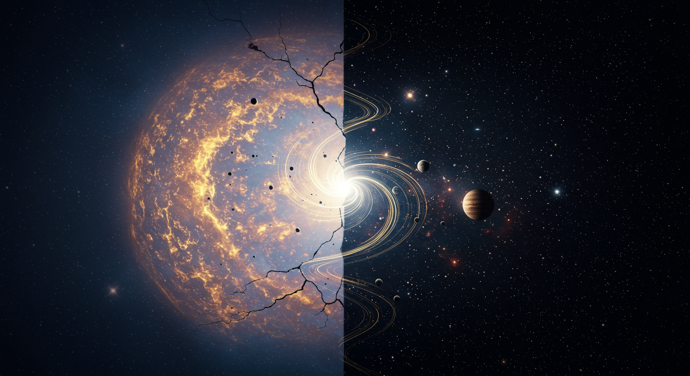
\begin{figure}[t]
\includegraphics[width=\linewidth]{NonRiemannianSchematic.pdf}
\caption{A schematic illustration of curvature~$\tensor{\RR}{_{\mu\nu\rho\sigma}}$ and torsion~$\tensor{\TT}{^{\alpha}_{\mu\nu}}$. The left of the diagram demonstrates curvature as taught in most introductions to GR: In the presence of curvature, the direction of vector changes when parallely transported around a loop. The right of the diagram illustrates torsion: In the presence of torsion, the infinitesimal parallelogram spanned by two vectors does not close.}
\label{fig:NonRiemannianSchematic}
\end{figure}
\paragraph*{Poincar\'e gauge theory} The gauge approach to gravity stands out among various theories of gravity, as gauge theories have been very successful in explaining the electroweak and strong sectors in particle physics, where forces are mediated by vector gauge bosons. Due to the importance of global Poincar\'e symmetry --- which includes four spacetime translations and the Lorentz group containing three spatial rotations and Lorentz boosts which rotate spacetime in three spatial directions --- the consideration of Poincaré gauge theory (PGT) arises naturally as a framework for describing the gravitational force~\cite{Utiyama:1956sy, Kibble:1961ba, Sciama:1964jqa, Hehl:1976kj}.
The gauge fields in PGT gauge the translational and rotational parts of the Poincaré group~\cite{Blagojevic:2002du}. The Lagrangian of PGT is built from the field strength tensors, one for each gauge field, which are identified with the torsion tensor~$\TT$, and the curvature tensor~$\RR$, respectively. The theory up to quadratic order in the curvature and torsion tensors with even parity has Lagrangian density~$\mathcal{L} \sim \RR + \RR^2 + \TT^2 + \mathcal{L}_\mathrm{M}$, where~$\mathcal{L}_\mathrm{M}$ is the matter Lagrangian. Whilst in GR,~$\RR^2$ operators are expected as one-loop corrections to the Einstein--Hilbert term in the presence of matter, in this paper, the quadratic Lagrangian structure is motivated by analogy to Yang--Mills theory since the same structures arise in the gauge theories of the SM. The specific model considered in this paper is purely of the form~$\RR^2 + \TT^2$, and it has been shown to be renormalizable by power counting~\cite{Lin:2018awc, Lin:2019ugq}.\footnote{As such, the full particle content of the theory is taken as being physical: new particles in~$\RR + \RR^2 +\TT^2$ theories which have been motivated as non-renormalisable effective field theories would instead be intrepreted as truncation artefacts~\cite{Glavan:2024cfs}.} As explained heuristically in~\cref{sec:perturbations} -- and shown in separate work~\cite{Barker:2025} -- the theory is expected to retain an Einsteinian limit even in the absence of the Einstein--Hilbert term. This is due to the post-Riemannian expansion of the Einstein--Cartan curvature, which gives rise to a cross-term~$\RR \TT^2$. Condensation of the torsion field at~$\TT^2 \sim \Mp$ leads to the emergence of the Einstein--Hilbert term.
\paragraph*{Torsion condensation (TorC)} The method of spin projection operators has been used to study PGT systematically, identifying parameter conditions that avoid unphysical ghost and tachyon degrees of freedom~\cite{Lin:2018awc, Lin:2019ugq}. The most developed among the resulting catalogue of models is the Torsion Condensation (TorC) model~\cite{Barker:2020elg, Barker:2020gcp, barker_2021, Rew:2023zxy}, with the Lagrangian density
\begin{equation}\label{eq:TorCLagrangian}
\begin{aligned}
\mathcal{L}_{\mathrm{TorC}} = & -\frac{4\Mp}{9} \tensor{\TT}{_\mu} \tensor{\TT}{^\mu} \\
& - \frac{\mu}{6} \Big[ \lambda \tensor{\TT}{_{\mu\nu\sigma}}\big( \tensor{\TT}{^{\mu\nu\sigma}} - 2 \tensor{\TT}{^{\nu\mu\sigma}} \big) \\
& + 12\tensor{\RR}{_{\mu\nu}} \big( \tensor{\RR}{^{[\mu\nu]}} - \tensor{\RR}{^{\mu\nu}} \big) \\
& - 2 \tensor{\RR}{_{\mu\nu\sigma\rho}} \big( \tensor{\RR}{^{\mu\nu\sigma\rho}} - 4 \tensor{\RR}{^{\mu\sigma\nu\rho}} - 5 \tensor{\RR}{^{\sigma\rho\mu\nu}} \big) \Big] \\
& + 2 \nu \tensor{\RR}{_{[\mu\nu]}} \tensor{\RR}{^{[\mu\nu]}} - \Mp \Lambda + \mathcal{L}_{\mathrm{M}},
\end{aligned}
\end{equation}
where~$\tensor{\RR}{_{\mu\nu\sigma\rho}}$ is the curvature, and~$\tensor{\TT}{^\mu_{\nu\sigma}}$ is the torsion tensor, with~$\tensor{\TT}{_\nu} \equiv \tensor{\TT}{^{\mu}_{\nu\mu}}$;~$\Mp = 1/8\pi G$ is the Planck mass,~$\nu$ and~$\mu$ are dimensionless curvature coupling constants;~$\lambda$ is a coupling constant of mass dimension two, which can be shown to give rise to a torsional dark energy term intrinsic to the gravitational sector, whereas~$\Lambda$ is the usual cosmological constant (which could also be absorbed into the matter Lagrangian~$\mathcal{L}_{\mathrm{M}}$). As shown in~\cref{sec:perturbations}, to ensure the absence of ghost and tachyon degrees of freedom in the tree-level perturbation theory, the following inequality must be satisfied~\cite{Lin:2019ugq}
\begin{equation}
\lambda \geq 0, \quad \mu < 0, \quad (\nu + 2 \mu)(\nu - \mu) > 0.
\label{eq:TorCconditions}
\end{equation}
For the purposes of this study, a further constraint
\begin{equation}
\lambda = 0,
\end{equation}
is imposed, which eliminates the torsional dark energy, reducing the dark energy sector to the standard cosmological constant,~$\Lambda$. Future work will explore the alternative scenario where $\lambda$ itelf drives cosmic acceleration, potentially eliminating the need for a cosmological constant.
An FLRW background is assumed, characterized by the line element
\begin{equation}
\mathrm{d}s^2 = -\mathrm{d}t^2 + a^2(t) \left(\frac{\mathrm{d}r^2}{1 - kr^2} + r^2 \mathrm{d}\Omega^2\right),
\end{equation}
where~$k$ is the dimensionful curvature parameter, and~$a(t)$ is the dimensionless scale factor of the Universe. It can be shown that the TorC field equations are insensitive to the value of~$k$, so that the expansion history is not affected by the actual closed, flat or open spatial geometry of the Universe. Therefore, a flat FLRW background is adopted throughout this work.
\paragraph*{Scalar-tensor equivalent of TorC} To explore the cosmology of TorC, an equivalent scalar-tensor formulation is introduced. Among the various gravity theories, those based on scalar fields within the framework of modified gravity are one of the most extensively explored models. Scalar-tensor theories involve the coupling of different scalar fields to the metric in a curved but torsion-free spacetime~\cite{Horndeski:1974wa}. Note that, in the absence of torsion, the non-Riemannian curvature~$\ECR{}$ becomes the usual Riemannian curvature~$\RiemannianR{}$ familiar from GR --- this matter is explained in detail in~\cref{sec:perturbations}. In the cosmological context, scalar fields offer the advantage of inducing accelerated expansion without necessarily violating the isotropy of the Universe,\footnote{This is in contrast to vector models, which always `point somewhere'; the condensation of a vector field to finite vacuum expectation value is generally understood to constitute an \ae{}ther~\cite{Skordis:2020eui, Hsu:2024ftc}.} making them compelling candidates for dark energy and early-Universe inflationary mechanisms. It has been shown that in a flat, homogeneous and isotropic Universe, the Lagrangian of PGT can be mapped to a bi-scalar-tensor theory~\cite{Barker:2020elg}. For TorC, the scalar-tensor equivalent Lagrangian density is
\begin{equation}\label{TorCLagrangianMA}
\begin{aligned}
\LTorC &= \Mp \Biggl[-\frac{2}{3} \Bigl(1-\frac{\varpi^2}{4}\Bigr) \RiemannianR{} + g^{\mu\nu} \partial_{\mu} \varpi \partial_{\nu} \varpi \\
&\ -\frac{4}{3} \sqrt{|J_{\mu } J^{\mu }|} - \phi^2 + \phi^2 \varpi^2 \Biggr] - \Mp \Lambda + \mathcal{L}_\mathrm{M}, \\
J_{\mu} &\equiv 4 \varpi^3 \partial_{\mu} (\phi/\varpi) + \partial_{\mu} \phi .
\end{aligned}
\end{equation}
In~\cref{TorCLagrangianMA}, both~$\varpi$ and~$\phi$ are scalar fields that arise naturally from the unique form adopted by torsion in a homogeneous and isotropic Universe~\cite{TSAMPARLIS197927},\footnote{Whilst~\cref{Tsamparlis} looks complicated, the principle for deriving it is very simple. The torsion tensor has index symmetry~$\TT{^\mu_{\nu\sigma}}=-\TT{^\mu_{\sigma\nu}}$. At the level of the background cosmology, the expanding Universe provides a preferred frame such that the index `0' corresponds to time experienced by observers embedded in the Hubble flow. Using this preferred direction~$\tensor*{\delta}{^\rho_0}$, there are only two tensor structures that can be present in~$\TT{^\mu_{\nu\sigma}}$, and these are parameterised by time-dependent scalar functions. The involved-looking normalisation of these scalars in~\cref{Tsamparlis}, and the shift involving the Hubble number, are purely for convenience in making sure that the modified Friedmann equations resulting from~\cref{TorCLagrangianMA} precisely match those of TorC. There is a formal way for deriving this general format for cosmological torsion using Lie derivatives~\cite{TSAMPARLIS197927} which, however, adds nothing of substance to the discussion.}
\begin{equation}\label{Tsamparlis}
\tensor{\TT}{^\mu_{\nu\sigma}}
= \tensor*{\delta}{^\rho_0} \left[ (\phi + 2H)\tensor*{\delta}{^\mu_{[\sigma}}\tensor{g}{_{\nu]\rho}}
- \sqrt{\frac{\Mp}{-3 \mu}}\varpi \tensor{\epsilon}{^\mu_{\rho\nu\sigma}} \right],
\end{equation}
where~$H(t)\equiv(\mathrm{d}a(t)/\mathrm{d}t)/a(t)$ is the Hubble parameter,~$\tensor{g}{_{\mu\nu}}$ is the metric tensor and~$\tensor{\epsilon}{^\mu_{\rho\nu\sigma}}$ is the totally antisymmetric tensor. A notable feature of the TorC model is that regardless of the value of the torsion scalar field~$\varpi$ in the early Universe, the field equations of TorC drive the scalar field towards unity~$\varpi \rightarrow 1$ as time progresses.\footnote{The~$\varpi$ field approaches the convenient value of unity due to the way in which it is normalised.} This is an attractor state in the dynamical system of the modified Friedmann equations, similar to how expanding de Sitter space is an attractor in GR when a cosmological constant is added. When the initial value of~$\varpi$ is set to be unity, the modified Friedmann equations of TorC become identical to those of GR at all future times, effectively reproducing the \LCDM{} model. The flexibility of this framework, however, allows for deviations from the \LCDM{} solution, effectively providing an extension to \LCDM{}. This offers a well-defined theoretical context for investigating possible resolutions to existing tensions in the \LCDM{} model, such as the Hubble tension. This work focuses on the background evolution of TorC cosmology and does not yet incorporate cosmological perturbations. For the purposes of this initial study, the perturbation equations remain those of standard \LCDM{}. Extending the framework to include TorC cosmological perturbations is an area of ongoing research.
\begin{table}[t]
\centering
\vspace{3mm}
\renewcommand{\arraystretch}{1.2}
\setlength{\tabcolsep}{6pt}
\begin{tabular}{c|l}
\toprule
PGT & Poincar\'e Gauge Theory\\
TorC & Torsion Condensation\\
CMB & Cosmic Microwave Background\\
\hline
SH0ES & Local~$H_0$ measurement from SH0ES (2020)~\cite{Riess:2020fzl}\\
Planck & Planck 2018 data release~\cite{Planck:2018vyg}\\
\botrule
\end{tabular}
\caption{A list of acronyms and the datasets used in this analysis.}
\end{table}
\paragraph*{In this paper} In this work, the cosmological implications of the TorC model are investigated, with particular attention given to its potential to alleviate the Hubble tension. TorC introduces two parameters beyond those in \LCDM{}: the early-Universe value of the torsion scalar field~$\varpi_r$ and its velocity, which may be `packaged' into the bare dark energy density parameter~$\Omega_L$. To constrain the TorC cosmological parameters, the nested sampling algorithm \texttt{PolyChord}~\cite{Handley:2015fda} is employed, interfaced via \texttt{Cobaya}~\cite{Torrado:2020dgo} with cosmological likelihoods and a modified version of \texttt{CAMB}~\cite{Lewis:1999bs}. A combined analysis is carried out between the Planck 2018 CMB data~\cite{Planck:2018vyg} and the 2020 SH0ES supernova measurement~\cite{Riess:2020fzl}, assessing the degree of tension between the two datasets using the~$R$-statistic~\cite{Handley:2019wlz, Hergt:2021qlh, Ormondroyd:2023cze}.
\paragraph*{Organisation of this paper} The paper is organized into the following sections: In~\cref{sec:cosmparam}, the two additional TorC parameters are introduced, along with their impact on the Universe's expansion history and the CMB power spectrum. In~\cref{sec:method}, the methodology for constraining the TorC parameters is outlined, including a description of prior choices and the likelihoods used in the analysis. Bayesian model comparison between \LCDM{} and TorC is also discussed, along with the tension statistics employed to assess the tension between datasets within the two models. In~\cref{sec:result}, the results of the parameter estimation are presented and compared to those obtained under the \LCDM{} model, in order to assess the viability of TorC as an alternative framework and its potential to resolve existing cosmological tensions. Finally, in~\cref{sec:conclusion}, the results are summarized, and the implications of the study are discussed, along with potential future directions of research.
\section{Cosmology}\label{sec:cosmparam}
\begin{table}[t]
\centering
\vspace{3mm}
\renewcommand{\arraystretch}{1.2}
\setlength{\tabcolsep}{6pt}
\begin{tabular}{c|l}
\toprule
~$\Omega_L$ & Bare dark energy density parameter\\
~$\varpi_r$ & Torsion scalar field value in the early Universe\\
\hline
$h$ & Dimensionless Hubble parameter\\
$\Omega_b$ & Baryon density parameter\\
$\Omega_c$ & Cold dark matter density parameter\\
$\tau_\mathrm{reio}$ & Reionisation optical depth\\
$A_s$ & Amplitude of primordial scalar power spectrum\\
$n_s$ & Primordial scalar spectral index\\
\botrule
\end{tabular}
\caption{Cosmological parameters of the TorC model. The top two rows list the two additional parameters introduced by TorC, while the bottom rows list the standard cosmological parameters in \LCDM{}.}
\label{tab:TorCparams}
\end{table}
The cosmology of TorC is explored under the assumption of a homogeneous and isotropic Universe. As an initial investigation, the scope of this work is restricted to the background evolution of TorC cosmology and does not consider cosmological perturbations. The perturbation equations therefore remain those of standard \LCDM{} throughout.
This section focuses on the two additional parameters introduced by the model:~$\Omega_L$, the bare dark energy density parameter, and~$\varpi_r$, specifying the value of the torsion scalar field in the early Universe, the list of cosmological parameters for TorC is presented in~\cref{tab:TorCparams}. In this section, their origin will be outlined:~$\Omega_L$ arises from the field equations of TorC, while~$\varpi_r$ is set as an initial condition required for solving them. TorC can be treated as an extension of \LCDM{} by absorbing the effects of~$\Omega_L$ and~$\varpi_r$ into an effective dark energy density and pressure. This reformulated dark energy is incorporated into a modified version of \texttt{CAMB} to investigate their impact on the CMB power spectrum.
\subsection{TorC cosmological parameters:~$\Omega_L$ and~$\varpi_r$}
Varying the scalar-tensor analogue of the TorC Lagrangian in~\cref{TorCLagrangianMA} with respect to the metric~$\tensor{g}{_{\mu\nu}}$ and scalar fields~$\varpi$ and~$\phi$ gives the modified Friedmann equations for TorC~\cite{Barker:2020elg}. The field equation of~$\phi$ reveals that it is not an independent variable, but can be expressed in terms of the other fields
\begin{equation}
\phi = \frac{2\bigl(\dot{a} \bigl(\varpi^2 -1\bigr) + a \varpi \dot{\varpi} \bigr) }{a \bigl(\varpi^2 -1\bigr)} ,
\end{equation}
where the derivative with respect to time is denoted by a dot, e.g.,~$\dot{a} \equiv \mathrm{d}a/\mathrm{d}t$. This property allows for the immediate algebraic elimination of~$\phi$ from the other field equations. The variation of the matter Lagrangian with respect to the metric functions yields the energy-momentum tensor of a perfect fluid, characterised by the energy density~$\rho$ and pressure~$P$, which includes contributions from the standard radiation and matter. We additionally absorb the effect of~$\Lambda$ into this stress-energy tensor, to account for dark energy. These quantities can be written in the form of density parameters as
\begin{subequations}
\begin{align}
\rho & = 3 \Mp H_0^2 (\Omega_r + \Omega_m + \Omega_L), \\
P & = 3 \Mp H_0^2 \left(\frac{\Omega_r}{3} - \Omega_L\right),
\end{align}
\end{subequations}
where~$H_0$ is the Hubble parameter today,~$\Omega_r$ and~$\Omega_m$ are the density parameters of radiation and matter, and~$\Omega_L$ represents the `intrinsic' dark energy density parameter, or the `bare' dark energy density parameter.
The field equations with respect to the two independent components of metric give analogues of the two Friedmann equations of GR, relating the content of the Universe to its expansion,
\begin{subequations}
\begin{align}
H^2 = & H_0^2 \frac{\Omega_r a^{-4}+\Omega_m a^{-3}+\Omega_L}{\varpi^2} \nonumber \\
& - \frac{\dot{\varpi} \left(6 H \varpi + \frac{\left(1+3\varpi^2\right)\dot{\varpi}}{\varpi^2-1}\right)}{3 \varpi^2}, \label{eq:TorCF1}\\
H^2 + \dot{H}^2 = & - H_0^2\frac{\Omega_r a^{-4} + \frac{1}{2}\Omega_m a^{-3} - \Omega_L}{\varpi^2}\nonumber\\
&- \frac{3 H \varpi \dot{\varpi} - \frac{(5+3 \varpi^2) \dot{\varpi} ^2}{\varpi -1} + 3 \varpi \ddot{\varpi}}{3 \varpi^2}, \label{eq:TorCF2}
\end{align}
\end{subequations}
The third equation is the equation of motion of the remaining torsion scalar field, describing the evolution of the torsion scalar field
\begin{align}
\ddot{\varpi} = & \frac{1}{\left(\varpi^2-1\right)\left(3 \varpi^2 +1\right)} \nonumber\\
&\times \Bigl( -3 \varpi \left(\varpi^2 -1\right)^2 \left(2 H^2 + \dot{H}\right) \nonumber\\
&+ 3 H \left(1 + 2 \varpi^2 - 3 \varpi^4\right) \dot{\varpi}\nonumber \\
& + 4 \varpi \dot{\varpi}^2 \Bigr).\label{eq:varpiEOM}
\end{align}
The analogue of the first Friedmann equation in~\cref{eq:TorCF1} is compared with the first Friedmann equation of the \LCDM{} model
\begin{equation}\label{eq:LCDMF1}
H^2 = H_0^2 \left(\Omega_r a^{-4} + \Omega_m a^{-3} + \Omega_{\Lambda} a^{-4}\right),
\end{equation}
where~$\Omega_{\Lambda}$ is the dark energy density parameter in \LCDM{}. It is evident that the equations~\cref{eq:TorCF1} and~\cref{eq:LCDMF1} differ in two key ways: first, the density parameters are effectively divided by~$\varpi^2$ in~\cref{eq:TorCF1}; second, an additional term appears in~\cref{eq:TorCF1}, involving the scale factor, torsion scalar field, and their derivatives. In standard \LCDM{}, the dark energy parameter~$\Omega_{\Lambda}$ is a constant that can be determined from the density parameters of the other components at~$a=1$ and~$H = H_0$, giving rise to the intuition that the non-gravitational energy budget of the Universe sums to unity when normalized. However, this relationship does not hold for TorC due to the presence of the extra term, similar to how a substantial curvature density would modify the Friedmann equations in GR. As a result,~$\Omega_L$ cannot be inferred from the other density parameters: it becomes an independent parameter of the model.
To determine the expansion history of the Universe and the evolution of the torsion scalar field, the field equations are solved numerically in conformal time~$\tau$ defined as
\begin{equation}
\mathrm{d}t = a \mathrm{d}\tau,
\end{equation}
using power series initial conditions for~$\varpi$ and~$a$ in the early Universe. As the bare dark energy density parameter~$\Omega_L$ plays a crucial role in shaping the late-time expansion of the Universe, it leads to a modified value of the current Hubble parameter~$H_0$. However, since~$H_0$ is a cosmological parameter fitted in the model, the scale factor~$a$ is normalized to ensure that the Hubble parameter reaches~$H_0$ at~$a=1$. This is implemented via a rescaling
\begin{equation}
a \rightarrow \alpha a,
\label{eq:rescale}
\end{equation}
where~$\alpha$ is a constant to be determined numerically.
The power series in the early Universe in~\cref{sec:TorCpower} reveals that the initial conditions for solving the system are functions of the early-Universe value of the torsion scalar field~$\varpi$, denoted~$\varpi_r$. In addition to~$\Omega_L$,~$\varpi_r$ thus emerges as an independent parameter of the model, playing a crucial role in early-Universe cosmology. The field equations of TorC thus introduce two new parameters,~$\Omega_L$ and~$\varpi_r$, which influence the expansion history of the TorC Universe.
\subsection{Effective dark energy density and pressure}\label{sec:effectiveDE}
As discussed in~\cref{sec:intro}, TorC reproduces the \LCDM{} model when~$\varpi$ is set to unity. In this limit, the derivatives of~$\varpi$ vanish, and the TorC field equations reduce to the Friedmann equations of \LCDM{}. Therefore, if one wishes to reproduce \LCDM{} throughout the whole history of the Universe, one only needs to set the initial value of~$\varpi$ to unity,~$\varpi_r = 1$, and the bare dark energy density parameter~$\Omega_L$ to its correspondent value in \LCDM{} model,~$\Omega_L = \Omega_\Lambda$. As \LCDM{} emerges as a particular dynamical evolution, based on a choice of initial conditions of the TorC model, TorC can be treated as an extension of \LCDM{}. The effect of the two additional parameters in TorC can be interpreted as deviations from the dark energy component of \LCDM{}. Rather than treating dark energy as a constant, it can be redefined as a time-dependent quantity, allowing the effects of the additional TorC terms to be absorbed into an evolving dark energy density and pressure. This reformulation enables the use of Boltzmann codes, such as \texttt{CAMB}, which are capable of incorporating modified dark energy models to investigate the impact of new parameters on the CMB power spectra. In this work, the treatment of dark energy is restricted to the background level, with effects of perturbation assumed to follow the standard \LCDM{}. The modified first Friedmann equation reflecting a time-dependent dark energy component takes the form
\begin{equation}
H^2 = H_0^2 \bigl(\Omega_r a^{-4} + \Omega_m a^{-3}\bigr) +\frac{\rho_{\Lambda}^{\mathrm{eff}}(t)}{3 \Mp}.
\label{eq:F1eff}
\end{equation}
By comparing~\cref{eq:F1eff} with~\cref{eq:TorCF1}, the additional terms in the TorC field equations can be reinterpreted as an effective dark energy density.
The effective dark energy density can be expressed as
\begin{align}
\rho_{\Lambda}^{\mathrm{eff}} \equiv \frac{3\Mp}{\varpi^2} \Biggl[ &H_0^2 \Omega_L - H_0^2\left(\varpi^2 -1\right)\left(\Omega_r a^{-4}+\Omega_m a^{-3}\right) \nonumber\\
& - 2 H \varpi \dot{\varpi} -\frac{\left(1+3 \varpi^2\right) \dot{\varpi}^2}{3\left(\varpi^2-1\right)}\Biggr].\label{eq:effrho}
\end{align}
Note that since the density parameters in~\cref{eq:TorCF1} are divided by~$\varpi^2$, they also appear in the effective dark energy density, as they cannot be isolated independently from~$\varpi$. The pressure of effective dark energy can then be obtained from the derivative of its density using the continuity equation\footnote{The assumption that effective fluid obeys a continuity equation follows precisely from the fact that the modified Friedmann equations are partitioned into a standard GR-like part and an effective modified gravity part. The continuity equation may then be derived purely due to the structure of the GR-like part: in turn this is a result of the Bianchi identity in GR, which forces the conservation of the stress-energy tensor to which gravity is coupled.}
\begin{equation}
\dot{\rho} = -3 H \left(\rho + P\right).
\end{equation}
We thus obtain the following expression for the effective dark energy pressure
\begin{samepage}
\begin{align}
P_{\Lambda}^\mathrm{eff} =& \frac{\Mp}{12 a^4 H \varpi^3(\varpi^2-1)}\Biggl[ 3 H_0^2 H \varpi \left(\varpi^2-1\right)\nonumber \\
& \times \Bigl(\Omega_r \bigl(\varpi^2 -1\bigr) - 3 a^4 \Omega_L \bigl(1 + 3\varpi^2 \bigr) \Bigr) \nonumber\\
& - 9 a^4 H^3 \varpi^3 \bigl(\varpi^2 -1\bigr)^2 \nonumber\\
& + 6 \bigl(\varpi^2 -1\bigr) \dot{\varpi} \biggl(4 H_0^2 \bigl(\Omega_r + \Omega_m a + \Omega_L a^4 \bigr) \nonumber\\
& -a^4 H^2 \varpi^2 \bigl(5 + 3 \varpi^2 \bigr)\biggr) \nonumber\\
& - 3 a^4 H \varpi \dot{\varpi}^2 \bigl(-13 + 3\varpi^2 \bigl(6 + \varpi^2\bigr)\bigr)\nonumber\\
& - 8 a^4 \bigl(1 + 3\varpi^2\bigr) \dot{\varpi}^3 \Biggr].\label{eq:effP}
\end{align}
\end{samepage}
The effect of~$\Omega_L$ and~$\varpi_r$ are thus absorbed into the effective dark energy density and pressure as a modification of time-dependent dark energy. By combining~\cref{eq:TorCF2,eq:varpiEOM}, one obtains a coupled system that governs the evolution of the torsion scalar field~$\varpi$ and the Hubble parameter. The equation of motion for~$\varpi$ determines how the scalar field evolves with time, while the modified Friedmann equation evolves the Hubble parameter, with each depending on the time-dependent values of the other. Together, these form an autonomous and self-consistent dynamical system: given suitable initial conditions, they can be solved simultaneously as a system of ordinary differential equations. This provides the evolution of~$\varpi$, its derivative, the Hubble parameter, and the scale factor. These solutions can then be substituted into the expressions for the time-dependent dark energy density and pressure in~\cref{eq:effrho,eq:effP}, yielding a complete description of cosmological evolution in the TorC framework. This allows for the exploration of their effects on the expansion history of the Universe and the CMB power spectra.
\subsection{Cosmological effects of~$\Omega_L$ and~$\varpi_r$}
\label{sec:effects}
\begin{figure*}[!htbp]
\centering
\includegraphics[width=\textwidth]{OmL_combined_H_CMB.pdf}
\caption{The effect of~$\Omega_L$ on the comoving Hubble horizon on the left and the CMB power spectrum on the right. The color bar indicates the value of~$\Omega_L$ in both panels. For both plots, the value for~$\varpi_r \sim 1$ is set as the \LCDM{}-equivalent case. The cosmological parameters for computing CMB power spectra are set as the \LCDM{} values based on Planck results~\cite{Planck:2018vyg}. For comparison, the case for GR (based on~$\Omega_r = 9.22 \times 10^{-5}$,~$\Omega_m = 0.314$ and~$H_0 = 67.4$ km/s/Mpc) is shown in the plots. A smaller value of~$\Omega_L$ results in a smaller comoving Hubble horizon at late matter-dominated epochs, increases the amplitude of the CMB power spectrum, and shifts the peaks to lower multipoles. }
\label{fig:OmLPlots}
\end{figure*}
\begin{figure*}[!htbp]
\centering
\includegraphics[width=\textwidth]{cpr_combined_H_CMB.pdf}
\caption{The effect of~$\varpi_r$ on the Comoving Hubble Horizon on the left and the CMB power spectrum on the right. The color bar indicates the value of~$\varpi_r$ in both panels. For both plots, the value for~$\Omega_L \sim 0.685$ is set as the \LCDM{}-equivalent case~\cite{Planck:2018vyg}. The other cosmological parameters are set as the values of the \LCDM{} model. For comparison, the case for GR (based on~$\Omega_r = 9.22 \times 10^{-5}$,~$\Omega_m = 0.314$ and~$H_0 = 67.4$ km/s/Mpc) is shown in the plots. A smaller value of~$\varpi_r$ results in a smaller comoving Hubble horizon at early radiation-dominated epoch, increases the amplitude of the CMB power spectrum, and shifts the peaks to higher multipoles. }
\label{fig:VarpirPlots}
\end{figure*}
To investigate the impact of the new TorC parameters on the CMB power spectrum, the model is treated as an extension of \LCDM{} and implemented with the \texttt{CAMB} Boltzmann code. \texttt{CAMB} computes the CMB power spectra for a given cosmological model and supports a range of dark energy scenarios by allowing modifications to the dark energy equation of state $w_\Lambda^\mathrm{eff} \equiv P_\Lambda^\mathrm{eff}/\rho_\Lambda^\mathrm{eff}$. However, attempting to incorporate the TorC extension through the equation of state $w_\Lambda^\mathrm{eff}(a)$ introduces poles when the dark energy density changes sign, as when~$\varpi$ exceeds unity in~\cref{eq:effrho}, the second and fourth terms become negative, potentially leading to a negative dark energy density during certain parts of the Universe’s evolution. This obstructs exploration of the full parameter space of~$\Omega_L$ and~$\varpi_r$. However, the issue arises only when using $w_\Lambda^\mathrm{eff}$, and is resolved when pressure and density are implemented separately. To address this, \texttt{CAMB} was therefore modified to evolve the system using the effective dark energy density and pressure directly\footnote{Modified \texttt{CAMB} to read external dark energy density and pressure:~\cite{ModifiedCAMB}.}.
\paragraph*{Effects of bare dark energy}~\Cref{fig:OmLPlots} shows the cosmological effects of~$\Omega_L$. Note that this procesure -- adjusting bare dark energy density while holding the other parameters fixed -- is not possible in \LCDM{} as the density parameters have to sum up to unity. The left panel demonstrates that~$\Omega_L$ primarily influences the late-time expansion, with its effect most significant at late matter-dominated epochs, where a lower value of~$\Omega_L$ leads to a smaller comoving Hubble horizon. It's contribution to the Hubble horizon is negligible at early times, resulting in an evolution of the early Universe that closely resembles \LCDM{}. The right panel of~\cref{fig:OmLPlots} shows that a decrease in~$\Omega_L$ shifts the CMB acoustic peaks to lower multipoles ($\ell$) and enhances their amplitudes. A lower~$\Omega_L$ causes photon-electron decoupling to occur at higher redshifts. This results in a reduction in both the sound horizon,~$r^*$, and the angular diameter distance to the last scattering surface,~$D_A^*$. However, a more significant reduction in~$D_A^*$ leads to an increase in the angular scale of the sound horizon, defined as~$r^*/D_A^*$, thereby shifting the acoustic peaks toward lower~$\ell$ values. Additionally, the earlier decoupling prolongs the period of gravitational potential decay during the radiation-dominated era. This enhanced decay, via the early integrated Sachs-Wolfe (ISW) effect, injects additional energy into the photon-baryon fluid, amplifying the acoustic peak amplitudes.
\paragraph*{Effects of early torsion} The effects of~$\varpi_r$ on the Hubble horizon and CMB power spectrum are shown in~\cref{fig:VarpirPlots}. The left panel shows that a decreasing~$\varpi_r$ reduces the comoving Hubble horizon in the early Universe, while converging with \LCDM{} at late times. Correspondingly, the right panel shows that a smaller~$\varpi_r$ shifts the acoustic peaks to higher multipoles~$\ell$ and increases their amplitudes. This shift results from the reduced sound horizon at decoupling, which is a consequence of the smaller Hubble horizon at early times. This mechanism is phenomenologically similar to that of early dark energy models (EDE)~\cite{Poulin:2018cxd, Kamionkowski:2022pkx}. However, unlike many EDE models, which introduce a new scalar field and potential for phenomenological gain, the torsional field in TorC arises uniquely from the unitary and power-counting renormalizable gauging of the Poincar\'e group, providing a more fundamental motivation. Furthermore, the smaller early Hubble horizon intensifies gravitational potential decay during the radiation-dominated era, thereby enhancing the early ISW effect, which acts as an additional driving force for photon-baryon oscillations and boosts the peak amplitudes.
\section{Methods}\label{sec:method}
The previous sections introduced the two new parameters in TorC,~$\Omega_L$ and~$\varpi_r$, and their effects on the Hubble horizon and CMB power spectra of the TorC Universe. To find the posterior distribution of the cosmological parameters in TorC, the \texttt{Polychord}~\cite{Handley:2015vkr} nested sampling algorithm is employed to explore the parameter space of TorC cosmological parameters. The sampling is conducted using \texttt{Cobaya}~\cite{Torrado:2020dgo} which interfaces the \texttt{CAMB} Boltzmann solver with \texttt{Polychord} and relevant cosmological likelihoods. Note that this analysis modifies the background expansion in \texttt{CAMB} using the TorC effective dark energy density and pressure, while the perturbation equations remain those of standard \LCDM{}.\footnote{As a initial study, only the background evolution of TorC is being investigated, cosmological perturbation theory for TorC will be developed in future work.}
The two models, TorC and \LCDM{}, are compared using the Bayesian evidence,~$\mathcal{Z}$. The tension between the Planck and SH0ES datasets is then assessed using the~$R$-statistic, which quantifies the degree of tension and its potential alleviation when comparing the \LCDM{} and TorC models.
\subsection{Numerical implementation}
As discussed in~\cref{sec:effects}, to explore the full parameter space of $\Omega_L$ and $\varpi_r$, the \texttt{CAMB} Boltzmann code is modified to read in a tabulated input of dark energy density~$\rho_\Lambda(a)$, and pressure~$P_\Lambda(a)$ as functions of scale factor~$a$. The modified version is available at~\cite{ModifiedCAMB}. This customized \texttt{CAMB} is then linked to a modified \texttt{Cobaya} which reads the same external~$\rho_\Lambda(a)$ and~$P_\Lambda(a)$, available at~\cite{ModifiedCobaya}.
The chains and supplementary files used to produce the plots and results presented in this paper are available at~\cite{ZenodoTorC}.
\subsection{Prior and likelihoods}
\label{sec:prior}
%
\begin{table}[t]
\centering
\vspace{3mm}
\renewcommand{\arraystretch}{1.2}
%\begin{tabularx}{\linewidth}{c|c}
\begin{tabularx}{\linewidth}{>{\centering\arraybackslash}X|>{\centering\arraybackslash}X}
\toprule
Parameter & Prior Range \\
\hline
~$\Omega_L$ &~$[0.1, 1.5]$ \\
~$\varpi_r$ &~$[0.1, 1.5]$ \\
\hline
~$h$ &~$[0.2, 1.0]$ \\
~$\Omega_b h^2$ &~$[0.005, 0.1]$ \\
~$\Omega_c h^2$ &~$[0.005, 0.99]$ \\
~$\tau_{\mathrm{reio}}$ &~$[0.01, 0.4]$ \\
~$n_s$ &~$[0.885, 1.04]$ \\
~$\log A_s$ &~$[2.5, 3.7]$ \\
\botrule
\end{tabularx}
\caption{Prior range for uniform priors on cosmological parameters in the TorC model and \LCDM{} model. The prior range for the \LCDM{} parameters comes from the default option in~\texttt{cobaya}.}
\label{tab:prior}
\end{table}
%
To explore the parameter space of the TorC model, uniform priors are adopted for the set of parameters~$\{\Omega_L$,~$\varpi_r$,~$h$,~$\Omega_b h^2$,~$\Omega_c h^2$,~$\tau_{\mathrm{reio}}$,~$n_s$,~$A_s\}$.~\footnote{The prior of~$\varpi_r$ is restricted to avoid singularity at~$\varpi_r = 1$, and a prior constraint is imposed on the total matter density, requiring~$\Omega_m = \Omega_b + \Omega_c < 1$ to avoid segmentation faults.} The last six parameters correspond to the standard cosmological parameters in the \LCDM{} model. The prior ranges for the cosmological parameters are summarized in~\cref{tab:prior}.
The likelihoods used in this study include the Planck 2018 high-$\ell$ and low-$\ell$ TT, TE, EE, and lensing likelihoods~\cite{Aghanim:2019ame}. Additionally, the 2020 SH0ES measurement of the present-day Hubble parameter,~$H_0 = 73.04 \pm 1.04$ \hunit~\cite{Riess:2020fzl}, is also included via a likelihood with a Gaussian profile in the parameter~$H_0$, enabling comparison between the two datasets and combined analysis. These likelihoods and priors are applied to both the TorC and \LCDM{} analysis.
\subsection{Bayesian model comparison}
Bayesian model comparison between TorC and \LCDM{} is conducted using the Bayesian evidence
\begin{equation}
\mathcal{Z} = \int \mathcal{L}(\theta) \pi(\theta) \mathrm{d}\theta,
\end{equation}
where~$\mathcal{L}(\theta)$ is the likelihood function given the model parameters~$\theta$, and~$\pi(\theta)$ is the prior probabilities. The evidence naturally incorporates `\emph{Occam's razor}', penalizing overly complex models. To better understand this, the evidence can be decomposed into two components in the logarithmic form~\cite{Handley:2015vkr, Balan:2024cmq}
\begin{equation}
\log \mathcal{Z} = \langle \log \mathcal{L}(\theta) \rangle - D_{KL}.
\end{equation}
The first term is the posterior-weighted log likelihood,
\begin{equation}
\langle \log \mathcal{L}(\theta) \rangle = \int \log \mathcal{L}(\theta) P(\theta | D) \mathrm{d}\theta,
\end{equation}
where~$P(\theta | D)$ is the posterior distribution of the parameters given the data~$D$. This term measures how well the model fits the data, averaged over the posterior distribution of the parameters. A larger value of this indicates that the model provides a better fit to the data.
The second term is the Kullback-Leibler (KL) divergence~\cite{Handley:2019pqx, Kullback:1951zyt}
\begin{equation}
D_{KL} = \int P(\theta | D) \log \frac{P(\theta | D)}{\pi(\theta)} \mathrm{d}\theta,
\end{equation}
which quantifies how much the posterior distribution has contracted relative to the prior. This term acts as a complexity penalty -- a model with a large parameter space that is significantly narrowed by the data will have a larger value of~$D_{KL}$.
For models~$M_1$ and~$M_2$, model comparison can be conducted using Bayes' theorem. Given uniform prior probabilities for the two models, the posterior probability $M_1$ is given by
\begin{equation}
P(M_1 | D) = \frac{\mathcal{Z}_1}{\mathcal{Z}_1 + \mathcal{Z}_2}.
\end{equation}
The ratio of posterior probability for the two model, $P(M_1 | D) / P(M_2 | D) = \mathcal{Z}_1 / \mathcal{Z}_2$, gives Bayes factor, which offers a direct measurement of the relative support for the two models, quantifying how much more strongly the data favors $M_1$ over $M_2$. In the logarithm form, the Bayes factor is given by
\begin{equation}
\begin{split}
\Delta \log \mathcal{Z} & = \log \mathcal{Z}_1 - \log \mathcal{Z}_2.\\
& = \Delta \langle \log \mathcal{L}(\theta) \rangle - \Delta D_{KL},
\end{split}
\label{eq:BayesFactor}
\end{equation}
values of~$\Delta \log \mathcal{Z} > 0$ indicate that $M_1$ is supported over $M_2$ by a factor of $\exp(\Delta \log \mathcal{Z})$, while~$\Delta \log \mathcal{Z} < 0$ suggests the opposite.
As shown in~\cref{eq:BayesFactor}, this framework allows the source of model preference to be identified, comparing the goodness-of-fit and the complexity penalty of the two models. This analysis will be performed between TorC and \LCDM{}, exploring the added complexity of the two new parameters~$\Omega_L$ and~$\varpi_r$ in TorC, and their impact on the fit to the datasets.
\subsection{Tension quantification}
The level of agreement between the Planck and SH0ES datasets is assessed using the~$R$-statistic with \texttt{anesthetic}~\cite{Handley:2019mfs}, which quantifies the relative confidence in one dataset given the other, compared to the confidence in the dataset given itself. For datasets $A$ and $B$, the~$R$-statistic is defined as
\begin{equation}
R = \frac{\mathcal{Z}_{AB}}{\mathcal{Z}_A \mathcal{Z}_B} = \frac{P(A, B)}{P(A)P(B)} = \frac{P(A|B)}{P(A)} = \frac{P(B|A)}{P(B)},
\end{equation}
where~$\mathcal{Z}_{AB}$ is the joint evidence for datasets~$A$ and~$B$, and~$\mathcal{Z}_A$ and~$\mathcal{Z}_B$ are the evidences for each dataset individually. For~$R \gg 1$, the two datasets are consistent, indicating that dataset~$B$ has strengthened our confidence in dataset~$A$ by a factor of~$R$. Conversely, for~$R \ll 1$, the two datasets are in tension.
For flat, uninformative priors, the~$R$-statistic becomes sensitive to prior volume. In such cases, increasing the prior range can artificially inflate~$R$, falsely suggesting greater agreement. This issue can be resolved by using the Bayesian suspiciousness metric~\cite{Handley:2019wlz}, which accounts for prior volume effects. In the present analysis, the~$R$-statistic is sufficient to assess the level of agreement between the two datasets.
\section{Results}\label{sec:result}
\Cref{fig:TorC_LCDM_posterior} shows the full posterior distributions of the TorC and \LCDM{} cosmological parameters. The result is obtained from \texttt{PolyChord} nested sampling with 1000 live points.
\begin{figure*}[!htbp]
\centering
\includegraphics[width=\textwidth]{TorC_LCDM_Full_Contour.pdf}
\caption{The figure shows the full posterior distributions of the cosmological parameters for \LCDM{} (Planck 2018 data [purple]) and TorC (Planck 2018 data [yellow] and joint Planck+SH0ES data [red]). Nested sampling was performed with \texttt{PolyChord} using 1000 live points, and the corner plot was generated with \texttt{anesthetic}. } \label{fig:TorC_LCDM_posterior}
\end{figure*}
\begin{figure*}[!htbp]
\centering
\begin{subfigure}{0.49\textwidth}
\centering
\includegraphics[width=\textwidth]{Omegam_H0_Contours.pdf}
\end{subfigure}
\hfill
\begin{subfigure}{0.49\textwidth}
\centering
\includegraphics[width=\textwidth]{TorC_Params_vs_H0.pdf}
\end{subfigure}
\caption{The left panel shows~$\Omega_m$-$H_0$ posterior contours for \LCDM{} (using Planck 2018 data [Purple], TRGB data [Orange]~\cite{Freedman:2020dne}, and SH0ES 2020 data [Blue]~\cite{Riess:2020fzl}) and for TorC (using Planck 2018 data [Yellow], and joint Planck and SH0ES data [Red]). The contours show the tension between the Planck and SH0ES posteriors in the \LCDM{} model, and the alleviation of this tension in the TorC model. The right panel shows the posterior distributions of the two TorC parameters~$\Omega_L$ and~$\varpi_r$ in the~$H_0$-plane. The plot shows a positive correlation between~$H_0$ and~$\Omega_L$, and a negative correlation between~$H_0$ and~$\varpi_r$. }
\label{fig:corners}
\end{figure*}
\subsection{$H_0$ Tension}
The TorC model is capable of alleviating the~$H_0$ tension by allowing for a higher inferred Hubble parameter compared to the \LCDM{} model. This is shown in the~$H_0$-$\Omega_m$ plane on the left panel of~\cref{fig:corners}. The \LCDM{} posteriors with Planck, SH0ES, and tip of the red giant branch (TRGB)~\cite{Freedman:2020dne} likelihoods reveal a clear tension between the Planck and SH0ES datasets. Whereas the TorC posteriors for both Planck likelihood alone and joint SH0ES and Planck likelihoods show a fit that is consistent with both datasets.
The right panel of~\cref{fig:corners} shows the posterior distributions of the two TorC parameters,~$\Omega_L$ and~$\varpi_r$, in the~$H_0$-plane. The~$H_0$-$\varpi_r$ plane shows a negative correlation: as~$\varpi_r$ decreases, the value of~$H_0$ increases. This behavior suggests that while the TorC model is consistent with \LCDM{}, it allows for a higher value of~$H_0$ through the presence of torsion. Furthermore, the~$H_0$-$\Omega_L$ plane shows a positive correlation, indicating that a higher~$H_0$ value in TorC is achieved not only through a reduction in~$\varpi_r$, but also by an increase in the amount of bare dark energy~$\Omega_L$.
\subsection{On~$S_8$}
As shown in~\cref{fig:TorC_LCDM_posterior}, when including the Planck likelihood alone, the TorC posterior allows for lower values of~$S_8$ while being consistent with the \LCDM{} result. Including SH0ES likelihood shifts the TorC posterior nominally closer to the KiDS-1000 result,~$S_8 = 0.745 \pm 0.039$~\cite{KiDS:2020suj}. However, these results must be interpreted with caution, as the current analysis does not include TorC cosmological perturbations. It is also worth noting that the more recent KiDS-Legacy analysis shows that the~$S_8$ value is consistent with the result from Planck~\cite{Wright:2025xka}. In future work, the TorC model will be extended to include perturbation analysis, which may provide a more accurate prediction of~$S_8$.
\subsection{Model comparison}
\begin{figure*}[!htbp]
\centering
\includegraphics[width=\textwidth]{LogZ_LogR.pdf}
\caption{The left panel shows the logarithmic Bayes factor between \LCDM{} and TorC models using Planck data and the joint SH0ES and Planck data, defined as~$\Delta \log \mathcal{Z} = \log \mathcal{Z}_{\mathrm{TorC}} - \log \mathcal{Z}_{\LCDM{}}$.
The right panel shows the logarithmic~$R$-statistic between Planck and SH0ES datasets for \LCDM{} and TorC models.
In both cases the statistics are simulated with 1000 data points.
}
\label{fig:LogZLogR}
\end{figure*}
Bayesian model comparison between the TorC and \LCDM{} models was carried out using both the Planck data alone and the joint Planck and SH0ES datasets. The Bayes factors between the TorC and \LCDM{} models were computed using \texttt{PolyChord}, the results are shown in the left panel of~\cref{fig:LogZLogR}. The Bayes factor is defined as~$\Delta \log \mathcal{Z} = \log \mathcal{Z}_{\mathrm{TorC}} - \log \mathcal{Z}_{\LCDM}$ in this case.
Writing the logarithmic Bayes factor in the form of the second line of~\cref{eq:BayesFactor}, namely $\log \Delta \mathcal{Z} = \Delta \langle \log \mathcal{L}(\theta) \rangle - \Delta D_{KL}$, the result with Planck 2018 alone is
\begin{equation} \label{eq:LogZPlanck}
\begin{split}
\Delta \log \mathcal{Z}^{\mathrm{Planck}} &= -5.627 \pm 0.269 \\
&= 0.417 \pm 0.114 - 6.044 \pm 0.265,
\end{split}
\end{equation}
and with the joint Planck and SH0ES datasets is
\begin{equation} \label{eq:LogZPlanckSH0ES}
\begin{split}
\Delta \log \mathcal{Z}^\mathrm{joint} &= 0.725 \pm 0.280 \\
&= 6.792 \pm 0.113 - 6.071 \pm 0.263.
\end{split}
\end{equation}
In both cases, the relative KL divergence is essentially the same, reflecting the complexity penalty from the two additional parameters in TorC.~\Cref{sec:TorCprior} illustrates this penalty by showing the additional parameter space in TorC and the compression of the prior into the posterior, which is quantified by the KL divergence term.
For the Planck-only analysis in~\cref{eq:LogZPlanck}, there is a positive contribution from the likelihood term, however, this improvement in fit is outweighed by the complexity penalty, resulting in a strong evidence favouring \LCDM{} over TorC. In the joint Planck and SH0ES analysis in~\cref{eq:LogZPlanckSH0ES}, the likelihood term becomes larger, indicating that TorC provides an improved fit to the joint datasets. However, this improvement does not sufficiently offset the complexity penalty, leading to a Bayesian evidence for TorC that is only comparable to \LCDM{}. This suggests while TorC can accommodate both datasets, its additional complexity does not provide a decisive advantage over \LCDM{}.
\subsection{Tension analysis between datasets}
The tension between the Planck and SH0ES datasets is quantified using the~$R$-statistic, and a comparison of~$\log R$ values between the \LCDM{} and TorC models is presented in the right panel of~\cref{fig:LogZLogR}. The \LCDM{} model shows a significant tension between the two datasets ($\log R = -5.60 \pm 0.28$), while the TorC model suggests consistency between them ($\log R = 0.70 \pm 0.27$). This improvement in the~$R$-statistic for the TorC model demonstrates its ability to increase compatibility between the Planck and SH0ES datasets, quantifying the alleviation of the~$H_0$ tension.
\section{Conclusions}\label{sec:conclusion}
This study investigates the torsion condensation (TorC) model -- a gravitational gauge field theory with quadratic Lagrangian terms in torsion and curvature. The TorC cosmology can be studied as an extension of the \LCDM{} model, introducing two new parameters,~$\Omega_L$ and~$\varpi_r$, corresponding to the bare dark energy density and value of torsional scalar field in the early Universe, respectively. The effects of these new parameters on the Hubble horizon and CMB power spectra are explored. The constraints on the TorC cosmological parameters are then obtained using the \texttt{PolyChord} nested sampling algorithm, interfaced with the \texttt{CAMB} Boltzmann code and Planck and SH0ES likelihoods through \texttt{Cobaya}.~$H_0$ shows a negative correlation with~$\varpi_r$ and a positive correlation with~$\Omega_L$, indicating that an introduction of torsion in the gravitational sector can increase the value of~$H_0$. Tension analysis using the~$R$-statistic quantifies the alleviation of the tension between the Planck and SH0ES datasets in the TorC model, further demonstrating the ability of TorC to increase compatibility between the two datasets. However, model comparison between TorC and \LCDM{} using Bayes factors shows that TorC is not decisively favoured against \LCDM{}: the improvement in fit does not significantly offset the complexity penalty from the two additional TorC parameters. Nevertheless, this study demonstrates the potential of the TorC model to address the~$H_0$ tension, and motivates further investigation into the cosmological implications of extended gravitational theories.
Future work will extend the analysis of TorC parameters by incorporating other cosmological likelihoods, such as the recent DESI BAO dataset~\cite{DESI:2025zgx}. The present study assumes a vanishing torsional dark energy component,~$\lambda = 0$, future investigations will consider scenarios in which both bare and torsional contributions to dark energy are present. The inclusion of torsional dark energy may offer a natural explanation for the remarkably small observed value of the cosmological constant, the concept of torsion acting as a dynamical source for dark energy is also an active field of research in other extended gravity frameworks~\cite{Benisty:2021sul, Benisty:2022lhr}. This study is also conducted in the context of a flat Universe. Future work will also explore scenarios with non-zero spatial curvature. While the TorC field equations for background evolution are insensitive to the spatial curvature constant~$k$, spatial curvature can still manifest through its standard geometric effects on light propagation and large-scale structure. It will be investigated whether TorC under non-zero spatial curvature can alleviate the curvature tension observed in the \LCDM{} model. Finally, the development of a perturbation theory for TorC will enable a deeper exploration of the model impact on cosmic structure formation and the CMB.
\begin{acknowledgments}
The authors would like to thank Mike Hobson, Anthony Lasenby, Adam Ormondroyd, and Dily Ong for useful discussions. SL would like to thank the IBM colour blind friendly palette for the color scheme used in the figures, and Joe Pattison and Oscar O'Hara for their advice on making the plots more visually appealing. WB is grateful for the support of Girton College, Cambridge, Marie Skłodowska-Curie Actions and the Institute of Physics of the Czech Academy of Sciences.
This work used the DiRAC Data Intensive service~(CSD3 \href{www.csd3.cam.ac.uk}{www.csd3.cam.ac.uk}) at the University of Cambridge, managed by the University of Cambridge University Information Services on behalf of the STFC DiRAC HPC Facility~(\href{www.dirac.ac.uk}{www.dirac.ac.uk}). The DiRAC component of CSD3 at Cambridge was funded by BEIS, UKRI and STFC capital funding and STFC operations grants. DiRAC is part of the UKRI Digital Research Infrastructure. The authors acknowledge the use of \texttt{NumPy}~\cite{harris2020array}, \texttt{SciPy}~\cite{2020SciPy-NMeth}, and \texttt{Matplotlib}~\cite{Hunter:2007} for numerical computations and plotting, and \texttt{gemini-2.5-flash-preview-04-17} for the improvement of clarity of this paper.
\leavevmode
\paragraph*{Disclaimer} Co-funded by the European Union (Physics for Future -- Grant Agreement No. 101081515). Views and opinions expressed are however those of the author(s) only and do not necessarily reflect those of the European Union or European Research Executive Agency. Neither the European Union nor the granting authority can be held responsible for them.
\end{acknowledgments}
\bibliography{NotINSPIRE,paper_Qtorsion}
\appendix
\section{Condensation and perturbation}\label{sec:perturbations}
\paragraph*{Poincar\'e gauge theory} We introduce the tensor-like fields~$\tensor{e}{^i_\mu}$ and~$\tensor{e}{_i^\mu}$ as the components of the co-tetrad and tetrad fields, respectively. These fields are associated with Roman Lorentz (i.e. anholonomic, not associated with any coordinates) indices, whereas the Greek indices used hitherto throughout this paper are holonomic, i.e. corresponding to spacetime coordinates. We recover the standard spacetime metric from these fields using~$\tensor{e}{^i_\mu}\tensor{e}{^j_\nu}\tensor{\eta}{_{ij}}\equiv\tensor{g}{_{\mu\nu}}$ and the inverse~$\tensor{e}{_i^\mu}\tensor{e}{_j^\nu}\tensor{\eta}{^{ij}}\equiv\tensor{g}{^{\mu\nu}}$ with two identities~$\tensor{e}{^i_\mu}\tensor{e}{_i^\nu}\equiv\tensor*{\delta}{_\mu^\nu}$ and~$\tensor{e}{^i_\mu}\tensor{e}{_j^\mu}\equiv\tensor*{\delta}{_j^i}$ as extra kinematical restrictions on the components. We next introduce an independent spin connection field~$\tensor{\omega}{^{ij}_\mu}\equiv\tensor{\omega}{^{[ij]}_\mu}$. Equipped with these two sets of gauge fields, we can proceed to define the PGT torsion and PGT curvature as covariant field strengths
\begin{subequations}
\begin{align}
\ECT{^k_{ij}}&\equiv 2\tensor{e}{_i^\mu}\tensor{e}{_j^\nu}\big(\PD{_{[\mu|}}\tensor{e}{^k_{|\nu]}}+\tensor{\omega}{^k_{m[\mu|}}\tensor{e}{^m_{|\nu]}}\big),\label{PGTTorsion}
\\
\tensor{\mathcal{R}}{^{kl}_{ij}}&\equiv 2\tensor{e}{_i^\mu}\tensor{e}{_j^\nu}\big(\PD{_{[\mu|}}\tensor{\omega}{^{kl}_{|\nu]}}+\tensor{\omega}{^k_{m[\mu|}}\tensor{\omega}{^{ml}_{|\nu]}}\big).\label{PGTCurvature}
\end{align}
\end{subequations}
Here, covariance refers to the transformations of both fields under the action of the Poincar\'e group, which we do not show in detail. In brief, however, under spatial translations the Greek indices transform with the standard Jacobian matrices of coordinate diffeomorphisms, and under local Lorentz transformations the Roman indices are rotated by the Lorentz transformation matrix familiar from special relativity, whilst the spin connection undergoes an additional inhomogeneous transformation involving the four-gradient of this local Lorentz rotation matrix. The holonomic components of the torsion and curvature in~\cref{eq:TorCLagrangian} are related to the quantities in~\cref{PGTTorsion,PGTCurvature} through~$\ECT{^\alpha_{\mu}_{\nu}}\equiv\tensor{e}{^i_\mu}\tensor{e}{_k^\alpha}\tensor{e}{^j_\nu}\ECT{^k_{ij}}$ and~$\tensor{\mathcal{R}}{^\rho_\sigma_{\mu\nu}}\equiv\tensor{e}{^i_\mu}\tensor{e}{^j_\nu}\tensor{e}{_k^\rho}\tensor{e}{_l_\sigma}\tensor{\mathcal{R}}{^{k}_{lij}}$. In the weak-field regime near to Minkowski spacetime we take~$\tensor{\omega}{^{ij}_\mu}$ to be perturbatively small, and we define the \emph{exact} perturbation of the tetrad to be~$\tensor{e}{_i^\mu}\equiv\tensor*{\delta}{_i^\mu}+\tensor{f}{_i^\mu}$ --- note that this corresponds to the so-called `Kronecker' gauge choice of the Minkowski vacuum. It is easy to confirm that, at lowest order in the perturbations, the Greek and Roman indices become interchangeable. When we count components, we find that there are in total 16 degrees of freedom (d.o.f) in~$\tensor{f}{_i^\mu}$ and a further 24 d.o.f in~$\tensor{\omega}{^{ij}_\mu}$. As source currents conjugate to the tetrad perturbation~$\tensor{f}{_i^\mu}$ and spin connection~$\tensor{\omega}{^{ij}_\mu}$ we introduce the (asymmetric) stress-energy tensor of matter~$\tensor{\tau}{^i_\mu}$ and also the spin current of matter~$\tensor{\sigma}{_{ij}^\mu}$. These source currents have their origin in the matter Lagrangian, the form of which need not be specified.
\paragraph*{Post-Riemannian formulation} Whilst the gauge-theoretic structure of PGT is the motivating framework for the TorC model, it may not be the most familiar framework to the reader. Indeed, there is a conceptually far simpler way to work with the TorC model, whereby the theory is separated into those parts which depend on the same Riemannian geometry in which GR is formulated, and the \emph{post-Riemannian} parts which depend on the torsion. To make the comparison with textbook GR as seamless as possible, it is usual to formulate this \emph{post-Riemannian decomposition} in terms of the metric~$\tensor{g}{_{\mu\nu}}$ rather than the tetrad~$\tensor{e}{_i^\mu}$. The non-Riemannian (torsionful) curvature defined in~\cref{PGTCurvature} and illustrated in~\cref{fig:NonRiemannianSchematic} can be alternatively expressed in terms of the usual metric and coordinate indices, along with a torsionful affine connection~$\AffineConnection{^\rho_{\mu\nu}}$ as
\begin{align}
\tensor{\mathcal{R}}{^\rho_\sigma_{\mu\nu}} &\equiv 2\left(\tensor{\partial}{_{[\mu|}}\AffineConnection{^\rho_{|\nu]}_\sigma}+\AffineConnection{^\rho_{[\mu|}_\alpha}\AffineConnection{^\alpha_{|\nu]}_\sigma}\right) \,,\label{PostRiemannianCurvatureDef}
\end{align}
where the torsion defined in~\cref{PGTTorsion} and illustrated in~\cref{fig:NonRiemannianSchematic} may be alternatively defined via the affine connection itself as
\begin{equation}
\ECT{^\alpha_\mu_\nu} \equiv 2\AffineConnection{^\alpha_{[\mu\nu]}} \,. \label{PostRiemannianTorsionDef}
\end{equation}
Note that~\cref{PostRiemannianCurvatureDef,PostRiemannianTorsionDef} are definitions that one is more likely to find in introductory textbooks. The physical content of~\cref{eq:TorCLagrangian} does not change when one uses~\cref{PostRiemannianCurvatureDef,PostRiemannianTorsionDef} instead of~\cref{PGTCurvature,PGTTorsion}, so long as~$\tensor{g}{_{\mu\nu}}$ and~$\AffineConnection{^\mu_{\nu\sigma}}$ are used as fundamental fields instead of~$\tensor{e}{_i^\mu}$ and~$\tensor{\omega}{^{ij}_\mu}$, respectively. The use of the affine connection as a fundamental field is known as the \emph{Palatini} formulation of the theory. The Palatini approach is occasionally used for GR itself, but this is not the standard approach, and once again we seek to connect with the most standard formulation possible. To reach this final formulation, one can decompose the affine connection into a Riemannian part and a post-Riemannian (torsionful) part
\begin{equation}
\AffineConnection{^\rho_\mu_\nu} \equiv \LeviCivitaConnection{^\rho_\mu_\nu} + \frac{1}{2}\left(\ECT{^\rho_{\mu\nu}} - \ECT{_{\nu\mu}^\rho} + \ECT{_{\mu}^\rho_{\nu}}\right),\label{Contorsion}
\end{equation}
where~$\LeviCivitaConnection{^\nu_\mu_\rho}\equiv\tensor{g}{^{\nu\lambda}}\big(\PD{_{(\mu}}\tensor{g}{_{\rho)\lambda}}-\frac{1}{2}\PD{_{\lambda}}\tensor{g}{_{\mu\rho}}\big)$ is the familiar Levi--Civita connection, i.e. the usual Christoffel symbols. It is easy to check that~\cref{Contorsion,PostRiemannianTorsionDef} are mutually consistent. When~\cref{Contorsion} is plugged into~\cref{PostRiemannianCurvatureDef}, one obtains a long formula (the details of whose indices are not useful to our discussion) of the form
\begin{equation}\label{PRE}
\tensor{\mathcal{R}}{}\sim\RiemannianR{}+\ECT{}^2+\CD{}\ECT{},
\end{equation}
where~$\CD{}$ denotes the usual GR covariant derivative with connection~$\LeviCivitaConnection{^\nu_\mu_\rho}$ and where the Riemannian curvature tensor of GR is
\begin{align}
\RiemannianR{^\rho_\sigma_{\mu\nu}} &\equiv 2\left(\tensor{\partial}{_{[\mu|}}\LeviCivitaConnection{^\rho_{|\nu]}_\sigma}+\LeviCivitaConnection{^\rho_{[\mu|}_\alpha}\LeviCivitaConnection{^\alpha_{|\nu]}_\sigma}\right) \,.\label{RiemannianCurvatureDef}
\end{align}
One may plug the post-Riemannian expansion in~\cref{PRE} into~\cref{eq:TorCLagrangian} to obtain the TorC Lagrangian in its post-Riemannian form.
\paragraph*{Torsion condensation} The vastness of the resulting post-Riemannian expression, which contains very many terms but which takes the schematic form
\begin{equation}\label{PRELagrangian}
\begin{aligned}
\mathcal{L}_{\text{TorC}}&\sim
\mu\RiemannianR{}^2
+\mu\RiemannianR{}\ECT{}^2
+\mu\RiemannianR{}\CD{}\ECT{}
\\&\quad
+\mu\left(\CD{}\ECT{}\right)^2
+(\mu+\nu)\CD{}\ECT{}^2\ECT{}
\\&\quad
+\left(\Mp+\mu\lambda\right)\ECT{}^2
+(\mu+\nu)\ECT{}^4
\\&\quad
- \Mp \Lambda + \mathcal{L}_{\mathrm{M}}
,
\end{aligned}
\end{equation}
reflects the true non-linear richness of the TorC model as expressed its easiest-to-understand field variables~$\tensor{g}{_{\mu\nu}}$ and~$\ECT{^\mu_{\nu\sigma}}$. In essence, we see how TorC manifests as a gravity model in which the usual Riemannian curvature tensor is coupled in a highly non-minimal way to~$\ECT{^\mu_{\nu\sigma}}$, as if the latter were an exotic kind of matter field. One takes variations of~\cref{PRELagrangian} with respect to~$\tensor{g}{_{\mu\nu}}$ to obtain the (highly modified) Einstein field equations of TorC; in particular the metric variation of~$\mathcal{L}_{\mathrm{M}}$ leads to the stress-energy tensor~$\StressEnergyTensor{^{\mu\nu}}$ of actual matter (baryons and CDM). The variations of~\cref{PRELagrangian} with respect to~$\ECT{^\mu_{\nu\sigma}}$ lead to the torsion equations of motion; note that the torsion variation of~$\mathcal{L}_{\mathrm{M}}$ will be denoted presently by the current~$\TorsionSource{_\mu^{\nu\sigma}}$ --- unlike the matter spin tensor conjugate to the spin connection, and the so-called hypermomentum current conjugate to the affine connection, this torsion source current does not have a standard name in the literature. Regardless of this source current and its origins in the matter sector, the torsion dynamics in the gravity sector clearly tell us that torsion tends to condense at the vacuum expectation value~$\TT^2 \sim \Mp$. To see this easily from~\cref{PRELagrangian} note that the torsion has both a quadratic interaction and a quartic interaction. This feature is shared by the `sombrero' potential of the Higgs doublet, where it leads to electroweak symmetry breaking.\footnote{Note that we assume the separation of scales~$\Mp\gg\lambda$.} Heuristically, one may see how the Einstein--Hilbert-like limit emerges from infrared physics when this condensate is plugged back into~\cref{PRELagrangian}, by examining the second term, with the quadratic-curvature operators in the first term acting as short-distance corrections.
\paragraph*{Particle spectroscopy} The spectrum of gravitational perturbations exhibited by TorC around the torsion condensate is an area of active study, well beyond the scope of this initial work; this naturally includes the development of the associated theory of cosmological perturbations. The tree-level particle spectrum is, however, very well understood around Minkowski spacetime with \emph{vanishing} background torsion: it is the unitarity of this particle spectrum which single-handedly motivates parameter constraints in~\cref{eq:TorCconditions}, and so in this section we improve on~\cite{Lin:2019ugq} by re-deriving these constraints using modern methods.\footnote{Note that even these constraints may possibly be relaxed if TorC is proven to be inherently non-perturbative around the Minkowski background, a contingency which (unlike for standard, non-condensate models) would not jeapordise its phenomenological utility.} In order to determine the tree-level spectrum of the theory in~\cref{eq:TorCLagrangian}, we use the \textit{PSALTer} software~\cite{Barker:2024juc,Barker:2025qmw}. Let us start with the formulation of TorC as a PGT. A collection of completely general test source currents~$\tensor{\sigma}{_{ij}^\mu}$ and~$\tensor{\tau}{^i_\mu}$ are together introduced as the vector~$\mathsf{J}$, whilst the fields~$\tensor{f}{_i^\mu}$ and~$\tensor{\omega}{^{ij}_\mu}$ are denoted by another vector~$\zeta$, so that the whole matter Lagrangian is simply~$\mathcal{L}_{\text{M}}\sim\zeta^{\text{T}}\cdot\mathsf{J}$ when working to lowest order in perturbations. Basing ourselves in position space, it follows that the action corresponding to~\cref{eq:TorCLagrangian} can be expressed schematically in terms of these source and field vectors as
\begin{equation}\label{GenLag}
\mathcal{S}=\int\mathrm{d}^4x\ \zeta^{\text{T}}(x)\cdot\left[\mathsf{O}(\partial)\cdot\zeta(x)-\mathsf{J}(x)\right]+\mathcal{O}(\zeta^3),
\end{equation}
where the operator matrix~$\mathsf{O}(\partial)$ is termed the (linearized) \emph{wave operator}. This matrix corresponds to a tensor structure which is a polynomial of (up to) second order in the partial derivative~$\PD{_\mu}$. It is also parameterised by~$\mu$ and~$\nu$, along with~$\lambda$ and~$\Mp$. Working from this representation of the action, the saturated propagator derived from~\cref{GenLag} is extracted by moving over to momentum space via~$\PD{_\mu}\mapsto -i\tensor{k}{_\mu}$, before proceeding to `invert' the wave operator and sandwich it between the conserved sources according to the formula
\begin{equation}\label{Propagator}
\Pi(k)\equiv\mathsf{J}^\dagger(k)\cdot\mathsf{O}^{-1}(k)\cdot\mathsf{J}(k).
\end{equation}
As expected of a PGT (and especially true in the case of TorC, for which extra `accidental' symmetries appear in the linearisation) the model in~\cref{GenLag} turns out to feature various gauge invariances: this means that the supposed `inverse' in~\cref{Propagator} is not well defined owing to degeneracies in the matrix representation of the wave operator. As a general principle, the same gauge symmetries that are associated one-to-one with these degeneracies result in the presence of constraints on the physical values of the source currents. Thus, the consequence of the `sandwiching' procedure in~\cref{Propagator} is that the singular parts of the matrix inverse exactly cancel against the roots of the sources. Continuing to work in~$k$-space, standard methods in polology tell us how the locations of the poles in~$\Pi(k)$ describe the (squares of the) masses of eternal states. Specifically, real masses are needed for non-tachyonic (physical) particles. At the same time, the residue of~$\Pi(k)$ on each of the poles must be positive-definite in order for the state to not be a ghost. In the case of the massive quantum states, use of a spin-parity ($J^P$) basis is ideal for framing the problem of wave operator inversion in terms of basic linear algebra. In the case of massless states, on the other hand, spin is properly described by helicity quantum numbers. For the massless calculation the spectrum is computed by brute-force, using the individual components of the tensors. Whilst this component-level procedure is effective at extracting the number of polarisations and their corresponding unitarity conditions, the massless~$J$ and~$P$ numbers are not always apparent. The~$J^P$ modes contained within~$\tensor{f}{_i^\mu}$ and~$\tensor{\omega}{^{ij}_\mu}$ are shown in~\cref{FieldKinematicsTetradPerturbation,FieldKinematicsSpinConnection} respectively. The spectrograph in~\cref{ParticleSpectrographTorCPGT} is then produced automatically by feeding in the linearisation of the TorC Lagrangian density in~\cref{eq:TorCLagrangian} to the software. One can also perform the corresponding analysis of the post-Riemannian decomposed model in~\cref{PRELagrangian}, and this provides a reassuring cross-check. In this case, one uses the (exactly defined) metric perturbation~$\MetricPerturbation{_{\mu\nu}}\equiv\tensor{g}{_{\mu\nu}}-\tensor{\eta}{_{\mu\nu}}$ and small~$\ECT{^\mu_{\nu\sigma}}$ instead of~$\tensor{f}{_i^\mu}$ and~$\tensor{\omega}{^{ij}_\mu}$, and the sources are~$\StressEnergyTensor{^{\mu\nu}}$ and~$\TorsionSource{_\mu^{\nu\sigma}}$. The spectrograph in this case is shown in~\cref{ParticleSpectrographTorCECT}. The kinematics tables for the fields and their sources are shown in~\cref{FieldKinematicsMetricPerturbation,FieldKinematicsTPerturbation}. The sources used for this spectroscopy analyis can be found at~\cite{PSALTer}.
\begin{table*}[htbp]
\includegraphics[width=\linewidth]{FieldKinematicsTetradPerturbation.pdf}
\caption{Output generated by \textit{PSALTer}. Field kinematics of the tetrad perturbation~$\tensor{f}{_i^\nu}$ and its conjugate source current~$\tensor{\tau}{^i_\mu}$ --- physically interpreted as the asymmetric stress-energy tensor of the matter sector. Note that when working to lowest order in the perturbations, the Greek (coordinate) and Roman (Lorentz) indices are freely exchanged. The tetrad perturbation decomposes into irreducible parts under the action of the three-dimensional rotation group~$\mathrm{SO}(3)$. These correspond to states of definite spin~$J$ and parity~$P$ (collectively~$J^P$). This decomposition is made possible by the introduction of a preferred frame, i.e. a unit-timelike vector~$\tensor{n}{_{\mu}}\equiv\tensor{k}{_{\mu}}/\sqrt{\tensor{k}{^\nu}\tensor{k}{_\nu}}$, where~$\tensor{k}{_\mu}$ is the four-momentum of massive particles. These definitions are used in~\cref{ParticleSpectrographTorCPGT}.}
\label{FieldKinematicsTetradPerturbation}
\end{table*}
\begin{table*}[htbp]
\includegraphics[width=\linewidth]{FieldKinematicsSpinConnection.pdf}
\caption{Output generated by \textit{PSALTer}. Field kinematics of the spin connection~$\tensor{\omega}{^{ij}_\mu}\equiv\tensor{\omega}{^{[ij]}_\mu}$ and conjugate source~$\tensor{\sigma}{_{ij}^\mu}$ --- the spin current of matter. The principles behind the decomposition are precisely the same as in~\cref{FieldKinematicsTetradPerturbation}. These definitions are used in~\cref{ParticleSpectrographTorCPGT}.}
\label{FieldKinematicsSpinConnection}
\end{table*}
\begin{figure*}[htbp]
\includegraphics[width=\linewidth]{ParticleSpectrographTorCPGT.pdf}
\caption{Output generated by \textit{PSALTer}. The spectrograph of the theory defined by~\cref{eq:TorCLagrangian}. At the top, the (Fourier transformed) wave operator~$\mathsf{O}(k)$ from~\cref{GenLag} is displayed in the~$J^P$-representation defined in~\cref{FieldKinematicsTetradPerturbation,FieldKinematicsSpinConnection}. The~$J^P$ states are organised into diagonal blocks of~$J=0$,~$J=1$ and~$J=2$, and within each block into diagonal parity-preserving sectors of~$P=1$ (orange) and~$P=-1$ (purple), along with off-diagonal parity-violating blocks (teal). The Lagrangian in~\cref{eq:TorCLagrangian} does not contain any odd powers of the totally antisymmetric tensor, so there is no mixing between parities in this theory. The theory contains as many as 21 gauge generators: this far exceeds the 10 gauge generators common to all instances of Poincar\'e gauge theory. The gauge symmetries impose constraints on the source currents. The particle spectrum consists of two massless polarisations and one massive pseudoscalar particle (i.e.~$J^P=0^-$). In terms of the couplings in~\cref{eq:TorCLagrangian} the pseudoscalar has mass~$\sqrt{\lambda}$, so that it is not a tachyon if~$\lambda\geq 0$. Its pole residue indicates that it is not a ghost if~$\mu<0$. The residue of the massless pole (where~$p$ denotes the particle energy in some fiducial frame) then indicates a no-ghost condition of~$(\nu + 2 \mu)(\nu - \mu) > 0$. Together, these three unitarity conditions are consistent with those in~\cref{eq:TorCconditions}.}
\label{ParticleSpectrographTorCPGT}
\end{figure*}
\begin{table*}[htbp]
\includegraphics[width=\linewidth]{FieldKinematicsMetricPerturbation.pdf}
\caption{Output generated by \textit{PSALTer}. Field kinematics of the metric perturbation~$\MetricPerturbation{_{\mu\nu}}$ and conjugate source~$\StressEnergyTensor{^{\mu\nu}}$. Note that, compared to~\cref{FieldKinematicsTetradPerturbation}, the metric perturbation has six \emph{fewer} d.o.f, manifest as the loss of one~$1^+$ and one~$1^-$ modes, and owing to the fact that the tetrad is an asymmetric rank-two field, whilst the metric is symmetric. How is it possible that the physics is not lost by this reduction of the fundamental fields? The post-Riemannian metric formulation of TorC is, in some sense, a description of the PGT formulation of TorC in gauge-invariant variables. In these variables, the local symmetry of the theory under the Lorentz part of the Poincar\'e group becomes hidden, so that the only symmetry expected of~\cref{PRELagrangian} is diffeomorphism invariance as shared by GR (encoding the translational part of the Poincar\'e group). In other words, the metric does away with redundant (gauge) d.o.f in the tetrad. These definitions are used in~\cref{ParticleSpectrographTorCECT}.}
\label{FieldKinematicsMetricPerturbation}
\end{table*}
\begin{table*}[htbp]
\includegraphics[width=\linewidth]{FieldKinematicsTPerturbation.pdf}
\caption{Output generated by \textit{PSALTer}. Field kinematics of the torsional perturbation~$\ECT{^\mu_{\nu\sigma}}$ and conjugate source~$\TorsionSource{_\mu^{\nu\sigma}}$. Note that since the torsion field~$\ECT{^\mu_{\nu\sigma}}\equiv\ECT{^\mu_{[\nu\sigma]}}$ is antisymmetric, it has 24 independent d.o.f, which is the same as the number of d.o.f in the spin connection~$\tensor{\omega}{^{ij}_\mu}\equiv\tensor{\omega}{^{[ij]}_\mu}$. Thus, the~$J^P$ modes are basically `clones' of those in~\cref{FieldKinematicsSpinConnection}. These definitions are used in~\cref{ParticleSpectrographTorCECT}.}
\label{FieldKinematicsTPerturbation}
\end{table*}
\begin{figure*}[htbp]
\includegraphics[width=0.9\linewidth]{ParticleSpectrographTorCECT.pdf}
\caption{Output generated by \textit{PSALTer}. The spectrograph of the theory defined by~\cref{PRELagrangian}, i.e. the post-Riemannian formulation of TorC. Due to the elimination of redundant (gauge) field d.o.f in~\cref{FieldKinematicsMetricPerturbation}, the wave operator matrix is smaller than in~\cref{ParticleSpectrographTorCPGT}. To compensate, there are six \emph{fewer} gauge symmetries and corresponding source constraints (15 symmetry generators rather than 21, though this still exceeds the four expected diffeomeorphism generators due to the presence of accidental symmetries in the linearised theory). Despite these changes, the physical content of TorC is unchanged, namely the (measurable) pseudoscalar mass, the number of massless polarisations and the overall unitarity conditions. These conditions are consistent with those in~\cref{eq:TorCconditions,ParticleSpectrographTorCPGT}. See~\cref{FieldKinematicsMetricPerturbation,FieldKinematicsTPerturbation} for the definitions of the fields and sources used in this spectrograph.}
\label{ParticleSpectrographTorCECT}
\end{figure*}
\noindent\begin{minipage}[t]{0.48\textwidth}
\section{Initial conditions}\label{sec:TorCpower}
By writing~$a$ and~$\varpi$ as~$a = \sum_{i=1}^{n} C_i^a \tau^i$ and~$\varpi = \sum_{i=1}^{n} C_i^{\varpi} \tau^i$, one can substitute the power series ans\"atze into the TorC field equations to determine their coefficients, thereby fully specifying the early-time behaviour of both~$a$ and~$\varpi$. The solutions for the coefficients of the first few terms in these series are:
\begin{samepage}
\begin{subequations}
\begin{align}
a = & \frac{H_0 \sqrt{\Omega_r}}{\alpha \varpi_r}\tau + \frac{H_0^2 \Omega_m\bigl(3 \varpi_r^2 + 1\bigl)}{16 \alpha \varpi_r^2} \tau^2 \nonumber\\
& + \frac{5 H_0^3 \Omega_m^2 \bigl(\varpi_r^2-1\bigr)}{512 \alpha \varpi_r^3\sqrt{\Omega_r}} \tau^3 \nonumber\\
& + \frac{H_0^4 \bigl(\varpi_r^2-1\bigr) \bigl(27 \varpi_r^2 -121\bigr) \Omega_m^3}{49152 \alpha \varpi_r^4\Omega_r} \tau^4 \nonumber\\
& + \frac{H_0^5}{131720 \alpha \varpi_r^5 \Omega_r^{3/2}} \biggl(32768 \bigl(3 \varpi_r^2 + 1\bigr) \Omega_r^3 \Omega_L \nonumber\\
& - 49 \bigl(9 \varpi_r^4 - 29 \varpi_r^2 + 20 \bigr) \Omega_m^4 \biggr) \tau^5 + \mathcal{O}(\tau^6),
\label{eq:aPowerSeries}\\
\varpi = & \varpi_r - \frac{3 H_0 \bigl(\varpi_r^2-1\bigr)\Omega_m}{16 \sqrt{\Omega_r}} \tau \nonumber\\
& + \frac{H_0^2 \bigl(18 \varpi_r^4 - 5 \varpi_r^2 - 13 \bigr) \Omega_m^2}{512 \varpi_r \Omega_r} \tau^2 \nonumber\\
& + \frac{H_0^3 \bigl(-324 \varpi_r^6 + 45 \varpi_r^4 - 20 \varpi_r^2 + 299 \bigr) \Omega_m^3}{49152 \varpi_r^2 \Omega_r^{3/2}} \tau^3 \nonumber\\
& + \frac{H_0^4}{1310720 \varpi_r^3 \Omega_r^2} \biggl[- 98304 \Omega_r^3 \Omega_L \nonumber\\
& +\bigl(\varpi_r^2 -1\bigr) \biggl(\bigl(2 \varpi_r^2\bigl(810 (\varpi_r^2 + \varpi_r^4) + 731\bigr)\nonumber \\
& + 2327\bigr)\biggr) \Omega_m^4 \biggr] \tau^4 + \mathcal{O}(\tau^5).
\label{eq:varpiPowerSeries}
\end{align}
\end{subequations}
\end{samepage}
The parameter~$\varpi_r$ corresponds to the zeroth-order term in the power series of~$\varpi$. As such, the power series of~$a$ and~$\varpi$ are functions of~$\varpi_r$ and~$\tau$.
Note that the normalisation~$\alpha$ only affects the scale factor~$a$. To ensure the validity of the power series, the initial value of~$\tau$ used for numerical evolution is chosen to be sufficiently small such that the first term in the power series of~$a$ dominates over the second term
\begin{equation}
\tau_{\mathrm{ini}} = 10^{-6} \frac{16 \sqrt{\Omega_r} \varpi_r}{\Omega_m \bigl(3 \varpi_r^2 + 1\bigr) H_0}.
\end{equation}
At such an early time, it is clear that the system's evolution is primarily governed by the zeroth-order term in the power series expansion of the torsion scalar field,~$\varpi_r$.
\end{minipage}%
\hfill%
\begin{minipage}[t]{0.48\textwidth}
\section{Prior compression}\label{sec:TorCprior}
\begin{center}
\includegraphics[width=\linewidth]{cpr_OmL_KL.pdf}
\captionof{figure}{A comparison of prior [Blue] and posterior distributions for the TorC parameters~$\Omega_L$ and $\varpi_r$, using the Planck 2018 data [Yellow] and the joint Planck 2018 and SH0ES data [Red]. The prior distribution represents the additional parameter space introduced by TorC over the \LCDM{} model. The sharp compression into the posterior distribution illustrates the information gain, which is quantified by the KL divergence.}
\label{fig:TorCprior}
\end{center}
\end{minipage}
\end{document}
```
4. **Bibliographic Information:**
```bbl
%apsrev4-2.bst 2019-01-14 (MD) hand-edited version of apsrev4-1.bst
%Control: key (0)
%Control: author (8) initials jnrlst
%Control: editor formatted (1) identically to author
%Control: production of article title (0) allowed
%Control: page (0) single
%Control: year (1) truncated
%Control: production of eprint (0) enabled
\begin{thebibliography}{63}%
\makeatletter
\providecommand \@ifxundefined [1]{%
\@ifx{#1\undefined}
}%
\providecommand \@ifnum [1]{%
\ifnum #1\expandafter \@firstoftwo
\else \expandafter \@secondoftwo
\fi
}%
\providecommand \@ifx [1]{%
\ifx #1\expandafter \@firstoftwo
\else \expandafter \@secondoftwo
\fi
}%
\providecommand \natexlab [1]{#1}%
\providecommand \enquote [1]{``#1''}%
\providecommand \bibnamefont [1]{#1}%
\providecommand \bibfnamefont [1]{#1}%
\providecommand \citenamefont [1]{#1}%
\providecommand \href@noop [0]{\@secondoftwo}%
\providecommand \href [0]{\begingroup \@sanitize@url \@href}%
\providecommand \@href[1]{\@@startlink{#1}\@@href}%
\providecommand \@@href[1]{\endgroup#1\@@endlink}%
\providecommand \@sanitize@url [0]{\catcode `\\12\catcode `\$12\catcode
`\&12\catcode `\#12\catcode `\^12\catcode `\_12\catcode `\%12\relax}%
\providecommand \@@startlink[1]{}%
\providecommand \@@endlink[0]{}%
\providecommand \url [0]{\begingroup\@sanitize@url \@url }%
\providecommand \@url [1]{\endgroup\@href {#1}{\urlprefix }}%
\providecommand \urlprefix [0]{URL }%
\providecommand \Eprint [0]{\href }%
\providecommand \doibase [0]{https://doi.org/}%
\providecommand \selectlanguage [0]{\@gobble}%
\providecommand \bibinfo [0]{\@secondoftwo}%
\providecommand \bibfield [0]{\@secondoftwo}%
\providecommand \translation [1]{[#1]}%
\providecommand \BibitemOpen [0]{}%
\providecommand \bibitemStop [0]{}%
\providecommand \bibitemNoStop [0]{.\EOS\space}%
\providecommand \EOS [0]{\spacefactor3000\relax}%
\providecommand \BibitemShut [1]{\csname bibitem#1\endcsname}%
\let\auto@bib@innerbib\@empty
%
\bibitem [{\citenamefont {Sarkar}\ \emph {et~al.}(2009)\citenamefont {Sarkar},
\citenamefont {Yadav}, \citenamefont {Pandey},\ and\ \citenamefont
{Bharadwaj}}]{Sarkar_2009}%
\BibitemOpen
\bibfield {author} {\bibinfo {author} {\bibfnamefont {P.}~\bibnamefont
{Sarkar}}, \bibinfo {author} {\bibfnamefont {J.}~\bibnamefont {Yadav}},
\bibinfo {author} {\bibfnamefont {B.}~\bibnamefont {Pandey}},\ and\ \bibinfo
{author} {\bibfnamefont {S.}~\bibnamefont {Bharadwaj}},\ }\bibfield {title}
{\bibinfo {title} {The scale of homogeneity of the galaxy distribution in
sdss dr6},\ }\href {https://doi.org/10.1111/j.1745-3933.2009.00738.x}
{\bibfield {journal} {\bibinfo {journal} {Monthly Notices of the Royal
Astronomical Society: Letters}\ }\textbf {\bibinfo {volume} {399}},\ \bibinfo
{pages} {L128–L131} (\bibinfo {year} {2009})}\BibitemShut {NoStop}%
\bibitem [{\citenamefont {Scrimgeour}\ \emph {et~al.}(2012)\citenamefont
{Scrimgeour}, \citenamefont {Davis}, \citenamefont {Blake}, \citenamefont
{James}, \citenamefont {Poole}, \citenamefont {Staveley-Smith}, \citenamefont
{Brough}, \citenamefont {Colless}, \citenamefont {Contreras}, \citenamefont
{Couch}, \citenamefont {Croom}, \citenamefont {Croton}, \citenamefont
{Drinkwater}, \citenamefont {Forster}, \citenamefont {Gilbank}, \citenamefont
{Gladders}, \citenamefont {Glazebrook}, \citenamefont {Jelliffe},
\citenamefont {Jurek}, \citenamefont {Li}, \citenamefont {Madore},
\citenamefont {Martin}, \citenamefont {Pimbblet}, \citenamefont {Pracy},
\citenamefont {Sharp}, \citenamefont {Wisnioski}, \citenamefont {Woods},
\citenamefont {Wyder},\ and\ \citenamefont {Yee}}]{Scrimgeour_2012}%
\BibitemOpen
\bibfield {author} {\bibinfo {author} {\bibfnamefont {M.~I.}\ \bibnamefont
{Scrimgeour}}, \bibinfo {author} {\bibfnamefont {T.}~\bibnamefont {Davis}},
\bibinfo {author} {\bibfnamefont {C.}~\bibnamefont {Blake}}, \bibinfo
{author} {\bibfnamefont {J.~B.}\ \bibnamefont {James}}, \bibinfo {author}
{\bibfnamefont {G.~B.}\ \bibnamefont {Poole}}, \bibinfo {author}
{\bibfnamefont {L.}~\bibnamefont {Staveley-Smith}}, \bibinfo {author}
{\bibfnamefont {S.}~\bibnamefont {Brough}}, \bibinfo {author} {\bibfnamefont
{M.}~\bibnamefont {Colless}}, \bibinfo {author} {\bibfnamefont
{C.}~\bibnamefont {Contreras}}, \bibinfo {author} {\bibfnamefont
{W.}~\bibnamefont {Couch}}, \bibinfo {author} {\bibfnamefont
{S.}~\bibnamefont {Croom}}, \bibinfo {author} {\bibfnamefont
{D.}~\bibnamefont {Croton}}, \bibinfo {author} {\bibfnamefont {M.~J.}\
\bibnamefont {Drinkwater}}, \bibinfo {author} {\bibfnamefont
{K.}~\bibnamefont {Forster}}, \bibinfo {author} {\bibfnamefont
{D.}~\bibnamefont {Gilbank}}, \bibinfo {author} {\bibfnamefont
{M.}~\bibnamefont {Gladders}}, \bibinfo {author} {\bibfnamefont
{K.}~\bibnamefont {Glazebrook}}, \bibinfo {author} {\bibfnamefont
{B.}~\bibnamefont {Jelliffe}}, \bibinfo {author} {\bibfnamefont {R.~J.}\
\bibnamefont {Jurek}}, \bibinfo {author} {\bibfnamefont {I.-h.}\ \bibnamefont
{Li}}, \bibinfo {author} {\bibfnamefont {B.}~\bibnamefont {Madore}}, \bibinfo
{author} {\bibfnamefont {D.~C.}\ \bibnamefont {Martin}}, \bibinfo {author}
{\bibfnamefont {K.}~\bibnamefont {Pimbblet}}, \bibinfo {author}
{\bibfnamefont {M.}~\bibnamefont {Pracy}}, \bibinfo {author} {\bibfnamefont
{R.}~\bibnamefont {Sharp}}, \bibinfo {author} {\bibfnamefont
{E.}~\bibnamefont {Wisnioski}}, \bibinfo {author} {\bibfnamefont
{D.}~\bibnamefont {Woods}}, \bibinfo {author} {\bibfnamefont {T.~K.}\
\bibnamefont {Wyder}},\ and\ \bibinfo {author} {\bibfnamefont {H.~K.~C.}\
\bibnamefont {Yee}},\ }\bibfield {title} {\bibinfo {title} {The wigglez dark
energy survey: the transition to large-scale cosmic homogeneity: Cosmic
homogeneity in the wigglez survey},\ }\href
{https://doi.org/10.1111/j.1365-2966.2012.21402.x} {\bibfield {journal}
{\bibinfo {journal} {Monthly Notices of the Royal Astronomical Society}\
}\textbf {\bibinfo {volume} {425}},\ \bibinfo {pages} {116–134} (\bibinfo
{year} {2012})}\BibitemShut {NoStop}%
\bibitem [{\citenamefont {Page}\ \emph {et~al.}(2003)\citenamefont {Page} \emph
{et~al.}}]{WMAP:2003tof}%
\BibitemOpen
\bibfield {author} {\bibinfo {author} {\bibfnamefont {L.}~\bibnamefont
{Page}} \emph {et~al.} (\bibinfo {collaboration} {WMAP}),\ }\bibfield
{title} {\bibinfo {title} {{First year Wilkinson Microwave Anisotropy Probe
(WMAP) observations: Interpretation of the TT and TE angular power spectrum
peaks}},\ }\href {https://doi.org/10.1086/377224} {\bibfield {journal}
{\bibinfo {journal} {Astrophys. J. Suppl.}\ }\textbf {\bibinfo {volume}
{148}},\ \bibinfo {pages} {233} (\bibinfo {year} {2003})},\ \Eprint
{https://arxiv.org/abs/astro-ph/0302220} {arXiv:astro-ph/0302220}
\BibitemShut {NoStop}%
\bibitem [{\citenamefont {Cyburt}\ \emph {et~al.}(2016)\citenamefont {Cyburt},
\citenamefont {Fields}, \citenamefont {Olive},\ and\ \citenamefont
{Yeh}}]{Cyburt:2015mya}%
\BibitemOpen
\bibfield {author} {\bibinfo {author} {\bibfnamefont {R.~H.}\ \bibnamefont
{Cyburt}}, \bibinfo {author} {\bibfnamefont {B.~D.}\ \bibnamefont {Fields}},
\bibinfo {author} {\bibfnamefont {K.~A.}\ \bibnamefont {Olive}},\ and\
\bibinfo {author} {\bibfnamefont {T.-H.}\ \bibnamefont {Yeh}},\ }\bibfield
{title} {\bibinfo {title} {{Big Bang Nucleosynthesis: 2015}},\ }\href
{https://doi.org/10.1103/RevModPhys.88.015004} {\bibfield {journal}
{\bibinfo {journal} {Rev. Mod. Phys.}\ }\textbf {\bibinfo {volume} {88}},\
\bibinfo {pages} {015004} (\bibinfo {year} {2016})},\ \Eprint
{https://arxiv.org/abs/1505.01076} {arXiv:1505.01076 [astro-ph.CO]}
\BibitemShut {NoStop}%
\bibitem [{\citenamefont {Riess}\ \emph {et~al.}(2019)\citenamefont {Riess},
\citenamefont {Casertano}, \citenamefont {Yuan}, \citenamefont {Macri},\ and\
\citenamefont {Scolnic}}]{Riess:2019cxk}%
\BibitemOpen
\bibfield {author} {\bibinfo {author} {\bibfnamefont {A.~G.}\ \bibnamefont
{Riess}}, \bibinfo {author} {\bibfnamefont {S.}~\bibnamefont {Casertano}},
\bibinfo {author} {\bibfnamefont {W.}~\bibnamefont {Yuan}}, \bibinfo {author}
{\bibfnamefont {L.~M.}\ \bibnamefont {Macri}},\ and\ \bibinfo {author}
{\bibfnamefont {D.}~\bibnamefont {Scolnic}},\ }\bibfield {title} {\bibinfo
{title} {{Large Magellanic Cloud Cepheid Standards Provide a 1{\%} Foundation
for the Determination of the Hubble Constant and Stronger Evidence for
Physics beyond $\Lambda$CDM}},\ }\href
{https://doi.org/10.3847/1538-4357/ab1422} {\bibfield {journal} {\bibinfo
{journal} {Astrophys. J.}\ }\textbf {\bibinfo {volume} {876}},\ \bibinfo
{pages} {85} (\bibinfo {year} {2019})},\ \Eprint
{https://arxiv.org/abs/1903.07603} {arXiv:1903.07603 [astro-ph.CO]}
\BibitemShut {NoStop}%
\bibitem [{\citenamefont {Verde}\ \emph {et~al.}(2019)\citenamefont {Verde},
\citenamefont {Treu},\ and\ \citenamefont {Riess}}]{Verde:2019ivm}%
\BibitemOpen
\bibfield {author} {\bibinfo {author} {\bibfnamefont {L.}~\bibnamefont
{Verde}}, \bibinfo {author} {\bibfnamefont {T.}~\bibnamefont {Treu}},\ and\
\bibinfo {author} {\bibfnamefont {A.~G.}\ \bibnamefont {Riess}},\ }\bibfield
{title} {\bibinfo {title} {{Tensions between the Early and the Late
Universe}},\ }\href {https://doi.org/10.1038/s41550-019-0902-0} {\bibfield
{journal} {\bibinfo {journal} {Nature Astron.}\ }\textbf {\bibinfo {volume}
{3}},\ \bibinfo {pages} {891} (\bibinfo {year} {2019})},\ \Eprint
{https://arxiv.org/abs/1907.10625} {arXiv:1907.10625 [astro-ph.CO]}
\BibitemShut {NoStop}%
\bibitem [{\citenamefont {Di~Valentino}\ \emph {et~al.}(2021)\citenamefont
{Di~Valentino}, \citenamefont {Mena}, \citenamefont {Pan}, \citenamefont
{Visinelli}, \citenamefont {Yang}, \citenamefont {Melchiorri}, \citenamefont
{Mota}, \citenamefont {Riess},\ and\ \citenamefont
{Silk}}]{DiValentino:2021izs}%
\BibitemOpen
\bibfield {author} {\bibinfo {author} {\bibfnamefont {E.}~\bibnamefont
{Di~Valentino}}, \bibinfo {author} {\bibfnamefont {O.}~\bibnamefont {Mena}},
\bibinfo {author} {\bibfnamefont {S.}~\bibnamefont {Pan}}, \bibinfo {author}
{\bibfnamefont {L.}~\bibnamefont {Visinelli}}, \bibinfo {author}
{\bibfnamefont {W.}~\bibnamefont {Yang}}, \bibinfo {author} {\bibfnamefont
{A.}~\bibnamefont {Melchiorri}}, \bibinfo {author} {\bibfnamefont {D.~F.}\
\bibnamefont {Mota}}, \bibinfo {author} {\bibfnamefont {A.~G.}\ \bibnamefont
{Riess}},\ and\ \bibinfo {author} {\bibfnamefont {J.}~\bibnamefont {Silk}},\
}\bibfield {title} {\bibinfo {title} {{In the realm of the Hubble
tension{\textemdash}a review of solutions}},\ }\href
{https://doi.org/10.1088/1361-6382/ac086d} {\bibfield {journal} {\bibinfo
{journal} {Class. Quant. Grav.}\ }\textbf {\bibinfo {volume} {38}},\ \bibinfo
{pages} {153001} (\bibinfo {year} {2021})},\ \Eprint
{https://arxiv.org/abs/2103.01183} {arXiv:2103.01183 [astro-ph.CO]}
\BibitemShut {NoStop}%
\bibitem [{\citenamefont {Dainotti}\ \emph {et~al.}(2021)\citenamefont
{Dainotti}, \citenamefont {De~Simone}, \citenamefont {Schiavone},
\citenamefont {Montani}, \citenamefont {Rinaldi},\ and\ \citenamefont
{Lambiase}}]{Dainotti:2021pqg}%
\BibitemOpen
\bibfield {author} {\bibinfo {author} {\bibfnamefont {M.~G.}\ \bibnamefont
{Dainotti}}, \bibinfo {author} {\bibfnamefont {B.}~\bibnamefont {De~Simone}},
\bibinfo {author} {\bibfnamefont {T.}~\bibnamefont {Schiavone}}, \bibinfo
{author} {\bibfnamefont {G.}~\bibnamefont {Montani}}, \bibinfo {author}
{\bibfnamefont {E.}~\bibnamefont {Rinaldi}},\ and\ \bibinfo {author}
{\bibfnamefont {G.}~\bibnamefont {Lambiase}},\ }\bibfield {title} {\bibinfo
{title} {{On the Hubble constant tension in the SNe Ia Pantheon sample}},\
}\href {https://doi.org/10.3847/1538-4357/abeb73} {\bibfield {journal}
{\bibinfo {journal} {Astrophys. J.}\ }\textbf {\bibinfo {volume} {912}},\
\bibinfo {pages} {150} (\bibinfo {year} {2021})},\ \Eprint
{https://arxiv.org/abs/2103.02117} {arXiv:2103.02117 [astro-ph.CO]}
\BibitemShut {NoStop}%
\bibitem [{\citenamefont {Dainotti}\ \emph {et~al.}(2022)\citenamefont
{Dainotti}, \citenamefont {De~Simone}, \citenamefont {Schiavone},
\citenamefont {Montani}, \citenamefont {Rinaldi}, \citenamefont {Lambiase},
\citenamefont {Bogdan},\ and\ \citenamefont {Ugale}}]{Dainotti:2022bzg}%
\BibitemOpen
\bibfield {author} {\bibinfo {author} {\bibfnamefont {M.~G.}\ \bibnamefont
{Dainotti}}, \bibinfo {author} {\bibfnamefont {B.}~\bibnamefont {De~Simone}},
\bibinfo {author} {\bibfnamefont {T.}~\bibnamefont {Schiavone}}, \bibinfo
{author} {\bibfnamefont {G.}~\bibnamefont {Montani}}, \bibinfo {author}
{\bibfnamefont {E.}~\bibnamefont {Rinaldi}}, \bibinfo {author} {\bibfnamefont
{G.}~\bibnamefont {Lambiase}}, \bibinfo {author} {\bibfnamefont
{M.}~\bibnamefont {Bogdan}},\ and\ \bibinfo {author} {\bibfnamefont
{S.}~\bibnamefont {Ugale}},\ }\bibfield {title} {\bibinfo {title} {{On the
Evolution of the Hubble Constant with the SNe Ia Pantheon Sample and Baryon
Acoustic Oscillations: A Feasibility Study for GRB-Cosmology in 2030}},\
}\href {https://doi.org/10.3390/galaxies10010024} {\bibfield {journal}
{\bibinfo {journal} {Galaxies}\ }\textbf {\bibinfo {volume} {10}},\ \bibinfo
{pages} {24} (\bibinfo {year} {2022})},\ \Eprint
{https://arxiv.org/abs/2201.09848} {arXiv:2201.09848 [astro-ph.CO]}
\BibitemShut {NoStop}%
\bibitem [{\citenamefont {Dainotti}\ \emph {et~al.}(2025)\citenamefont
{Dainotti} \emph {et~al.}}]{Dainotti:2025qxz}%
\BibitemOpen
\bibfield {author} {\bibinfo {author} {\bibfnamefont {M.~G.}\ \bibnamefont
{Dainotti}} \emph {et~al.},\ }\bibfield {title} {\bibinfo {title} {{A New
Master Supernovae Ia sample and the investigation of the Hubble tension}},\
}\href {https://doi.org/10.1016/j.jheap.2025.100405} {\bibfield {journal}
{\bibinfo {journal} {JHEAp}\ }\textbf {\bibinfo {volume} {48}},\ \bibinfo
{pages} {100405} (\bibinfo {year} {2025})},\ \Eprint
{https://arxiv.org/abs/2501.11772} {arXiv:2501.11772 [astro-ph.CO]}
\BibitemShut {NoStop}%
\bibitem [{\citenamefont {Handley}(2021)}]{Handley:2019tkm}%
\BibitemOpen
\bibfield {author} {\bibinfo {author} {\bibfnamefont {W.}~\bibnamefont
{Handley}},\ }\bibfield {title} {\bibinfo {title} {{Curvature tension:
evidence for a closed universe}},\ }\href
{https://doi.org/10.1103/PhysRevD.103.L041301} {\bibfield {journal}
{\bibinfo {journal} {Phys. Rev. D}\ }\textbf {\bibinfo {volume} {103}},\
\bibinfo {pages} {L041301} (\bibinfo {year} {2021})},\ \Eprint
{https://arxiv.org/abs/1908.09139} {arXiv:1908.09139 [astro-ph.CO]}
\BibitemShut {NoStop}%
\bibitem [{\citenamefont {Di~Valentino}\ \emph {et~al.}(2019)\citenamefont
{Di~Valentino}, \citenamefont {Melchiorri},\ and\ \citenamefont
{Silk}}]{DiValentino:2019qzk}%
\BibitemOpen
\bibfield {author} {\bibinfo {author} {\bibfnamefont {E.}~\bibnamefont
{Di~Valentino}}, \bibinfo {author} {\bibfnamefont {A.}~\bibnamefont
{Melchiorri}},\ and\ \bibinfo {author} {\bibfnamefont {J.}~\bibnamefont
{Silk}},\ }\bibfield {title} {\bibinfo {title} {{Planck evidence for a
closed Universe and a possible crisis for cosmology}},\ }\href
{https://doi.org/10.1038/s41550-019-0906-9} {\bibfield {journal} {\bibinfo
{journal} {Nature Astron.}\ }\textbf {\bibinfo {volume} {4}},\ \bibinfo
{pages} {196} (\bibinfo {year} {2019})},\ \Eprint
{https://arxiv.org/abs/1911.02087} {arXiv:1911.02087 [astro-ph.CO]}
\BibitemShut {NoStop}%
\bibitem [{\citenamefont {Fields}\ \emph {et~al.}(2020)\citenamefont {Fields},
\citenamefont {Olive}, \citenamefont {Yeh},\ and\ \citenamefont
{Young}}]{Fields:2019pfx}%
\BibitemOpen
\bibfield {author} {\bibinfo {author} {\bibfnamefont {B.~D.}\ \bibnamefont
{Fields}}, \bibinfo {author} {\bibfnamefont {K.~A.}\ \bibnamefont {Olive}},
\bibinfo {author} {\bibfnamefont {T.-H.}\ \bibnamefont {Yeh}},\ and\ \bibinfo
{author} {\bibfnamefont {C.}~\bibnamefont {Young}},\ }\bibfield {title}
{\bibinfo {title} {{Big-Bang Nucleosynthesis after Planck}},\ }\href
{https://doi.org/10.1088/1475-7516/2020/03/010} {\bibfield {journal}
{\bibinfo {journal} {JCAP}\ }\textbf {\bibinfo {volume} {03}},\ \bibinfo
{pages} {010}},\ \bibinfo {note} {[Erratum: JCAP 11, E02 (2020)]},\ \Eprint
{https://arxiv.org/abs/1912.01132} {arXiv:1912.01132 [astro-ph.CO]}
\BibitemShut {NoStop}%
\bibitem [{\citenamefont {Donoghue}(1994)}]{Donoghue:1994dn}%
\BibitemOpen
\bibfield {author} {\bibinfo {author} {\bibfnamefont {J.~F.}\ \bibnamefont
{Donoghue}},\ }\bibfield {title} {\bibinfo {title} {{General relativity as
an effective field theory: The leading quantum corrections}},\ }\href
{https://doi.org/10.1103/PhysRevD.50.3874} {\bibfield {journal} {\bibinfo
{journal} {Phys. Rev. D}\ }\textbf {\bibinfo {volume} {50}},\ \bibinfo
{pages} {3874} (\bibinfo {year} {1994})},\ \Eprint
{https://arxiv.org/abs/gr-qc/9405057} {arXiv:gr-qc/9405057} \BibitemShut
{NoStop}%
\bibitem [{\citenamefont {De~Simone}\ \emph {et~al.}(2025)\citenamefont
{De~Simone}, \citenamefont {van Putten}, \citenamefont {Dainotti},\ and\
\citenamefont {Lambiase}}]{DeSimone:2024lvy}%
\BibitemOpen
\bibfield {author} {\bibinfo {author} {\bibfnamefont {B.}~\bibnamefont
{De~Simone}}, \bibinfo {author} {\bibfnamefont {M.~H. P.~M.}\ \bibnamefont
{van Putten}}, \bibinfo {author} {\bibfnamefont {M.~G.}\ \bibnamefont
{Dainotti}},\ and\ \bibinfo {author} {\bibfnamefont {G.}~\bibnamefont
{Lambiase}},\ }\bibfield {title} {\bibinfo {title} {{A doublet of
cosmological models to challenge the H0 tension in the Pantheon Supernovae Ia
catalog}},\ }\href {https://doi.org/10.1016/j.jheap.2024.12.003} {\bibfield
{journal} {\bibinfo {journal} {JHEAp}\ }\textbf {\bibinfo {volume} {45}},\
\bibinfo {pages} {290} (\bibinfo {year} {2025})},\ \Eprint
{https://arxiv.org/abs/2411.05744} {arXiv:2411.05744 [astro-ph.CO]}
\BibitemShut {NoStop}%
\bibitem [{\citenamefont {Utiyama}(1956)}]{Utiyama:1956sy}%
\BibitemOpen
\bibfield {author} {\bibinfo {author} {\bibfnamefont {R.}~\bibnamefont
{Utiyama}},\ }\bibfield {title} {\bibinfo {title} {{Invariant theoretical
interpretation of interaction}},\ }\href
{https://doi.org/10.1103/PhysRev.101.1597} {\bibfield {journal} {\bibinfo
{journal} {Phys. Rev.}\ }\textbf {\bibinfo {volume} {101}},\ \bibinfo {pages}
{1597} (\bibinfo {year} {1956})}\BibitemShut {NoStop}%
\bibitem [{\citenamefont {Kibble}(1961)}]{Kibble:1961ba}%
\BibitemOpen
\bibfield {author} {\bibinfo {author} {\bibfnamefont {T.~W.~B.}\
\bibnamefont {Kibble}},\ }\bibfield {title} {\bibinfo {title} {{Lorentz
invariance and the gravitational field}},\ }\href
{https://doi.org/10.1063/1.1703702} {\bibfield {journal} {\bibinfo
{journal} {J. Math. Phys.}\ }\textbf {\bibinfo {volume} {2}},\ \bibinfo
{pages} {212} (\bibinfo {year} {1961})}\BibitemShut {NoStop}%
\bibitem [{\citenamefont {Sciama}(1964)}]{Sciama:1964jqa}%
\BibitemOpen
\bibfield {author} {\bibinfo {author} {\bibfnamefont {D.~W.}\ \bibnamefont
{Sciama}},\ }\bibfield {title} {\bibinfo {title} {{The Physical Structure of
General Relativity}},\ }\href {https://doi.org/10.1103/RevModPhys.36.463}
{\bibfield {journal} {\bibinfo {journal} {Rev. Mod. Phys.}\ }\textbf
{\bibinfo {volume} {36}},\ \bibinfo {pages} {463} (\bibinfo {year}
{1964})}\BibitemShut {NoStop}%
\bibitem [{\citenamefont {Hehl}\ \emph {et~al.}(1976)\citenamefont {Hehl},
\citenamefont {Von Der~Heyde}, \citenamefont {Kerlick},\ and\ \citenamefont
{Nester}}]{Hehl:1976kj}%
\BibitemOpen
\bibfield {author} {\bibinfo {author} {\bibfnamefont {F.~W.}\ \bibnamefont
{Hehl}}, \bibinfo {author} {\bibfnamefont {P.}~\bibnamefont {Von Der~Heyde}},
\bibinfo {author} {\bibfnamefont {G.~D.}\ \bibnamefont {Kerlick}},\ and\
\bibinfo {author} {\bibfnamefont {J.~M.}\ \bibnamefont {Nester}},\ }\bibfield
{title} {\bibinfo {title} {{General Relativity with Spin and Torsion:
Foundations and Prospects}},\ }\href
{https://doi.org/10.1103/RevModPhys.48.393} {\bibfield {journal} {\bibinfo
{journal} {Rev. Mod. Phys.}\ }\textbf {\bibinfo {volume} {48}},\ \bibinfo
{pages} {393} (\bibinfo {year} {1976})}\BibitemShut {NoStop}%
\bibitem [{\citenamefont {Blagojevic}(2002)}]{Blagojevic:2002du}%
\BibitemOpen
\bibfield {author} {\bibinfo {author} {\bibfnamefont {M.}~\bibnamefont
{Blagojevic}},\ }\href {https://doi.org/10.1201/9781420034264} {\emph
{\bibinfo {title} {{Gravitation and gauge symmetries}}}}\ (\bibinfo {year}
{2002})\BibitemShut {NoStop}%
\bibitem [{\citenamefont {Lin}\ \emph {et~al.}(2019)\citenamefont {Lin},
\citenamefont {Hobson},\ and\ \citenamefont {Lasenby}}]{Lin:2018awc}%
\BibitemOpen
\bibfield {author} {\bibinfo {author} {\bibfnamefont {Y.-C.}\ \bibnamefont
{Lin}}, \bibinfo {author} {\bibfnamefont {M.~P.}\ \bibnamefont {Hobson}},\
and\ \bibinfo {author} {\bibfnamefont {A.~N.}\ \bibnamefont {Lasenby}},\
}\bibfield {title} {\bibinfo {title} {{Ghost and tachyon free Poincar{\'e}
gauge theories: A systematic approach}},\ }\href
{https://doi.org/10.1103/PhysRevD.99.064001} {\bibfield {journal} {\bibinfo
{journal} {Phys. Rev. D}\ }\textbf {\bibinfo {volume} {99}},\ \bibinfo
{pages} {064001} (\bibinfo {year} {2019})},\ \Eprint
{https://arxiv.org/abs/1812.02675} {arXiv:1812.02675 [gr-qc]} \BibitemShut
{NoStop}%
\bibitem [{\citenamefont {Lin}\ \emph {et~al.}(2020)\citenamefont {Lin},
\citenamefont {Hobson},\ and\ \citenamefont {Lasenby}}]{Lin:2019ugq}%
\BibitemOpen
\bibfield {author} {\bibinfo {author} {\bibfnamefont {Y.-C.}\ \bibnamefont
{Lin}}, \bibinfo {author} {\bibfnamefont {M.~P.}\ \bibnamefont {Hobson}},\
and\ \bibinfo {author} {\bibfnamefont {A.~N.}\ \bibnamefont {Lasenby}},\
}\bibfield {title} {\bibinfo {title} {{Power-counting renormalizable,
ghost-and-tachyon-free Poincar{\'e} gauge theories}},\ }\href
{https://doi.org/10.1103/PhysRevD.101.064038} {\bibfield {journal} {\bibinfo
{journal} {Phys. Rev. D}\ }\textbf {\bibinfo {volume} {101}},\ \bibinfo
{pages} {064038} (\bibinfo {year} {2020})},\ \Eprint
{https://arxiv.org/abs/1910.14197} {arXiv:1910.14197 [gr-qc]} \BibitemShut
{NoStop}%
\bibitem [{\citenamefont {Glavan}\ \emph {et~al.}(2025)\citenamefont {Glavan},
\citenamefont {Mukohyama},\ and\ \citenamefont {Zlosnik}}]{Glavan:2024cfs}%
\BibitemOpen
\bibfield {author} {\bibinfo {author} {\bibfnamefont {D.}~\bibnamefont
{Glavan}}, \bibinfo {author} {\bibfnamefont {S.}~\bibnamefont {Mukohyama}},\
and\ \bibinfo {author} {\bibfnamefont {T.}~\bibnamefont {Zlosnik}},\
}\bibfield {title} {\bibinfo {title} {{Removing spurious degrees of freedom
from EFT of gravity}},\ }\href
{https://doi.org/10.1088/1475-7516/2025/01/111} {\bibfield {journal}
{\bibinfo {journal} {JCAP}\ }\textbf {\bibinfo {volume} {01}},\ \bibinfo
{pages} {111}},\ \Eprint {https://arxiv.org/abs/2409.15989} {arXiv:2409.15989
[gr-qc]} \BibitemShut {NoStop}%
\bibitem [{\citenamefont {Barker}\ \emph
{et~al.}(2025{\natexlab{a}})\citenamefont {Barker}, \citenamefont {Lasenby},\
and\ \citenamefont {Hobson}}]{Barker:2025}%
\BibitemOpen
\bibfield {author} {\bibinfo {author} {\bibfnamefont {W.}~\bibnamefont
{Barker}}, \bibinfo {author} {\bibfnamefont {A.}~\bibnamefont {Lasenby}},\
and\ \bibinfo {author} {\bibfnamefont {M.}~\bibnamefont {Hobson}},\
}\bibfield {title} {\bibinfo {title} {{In preparation}},\ }\href@noop {} {\
(\bibinfo {year} {2025}{\natexlab{a}})}\BibitemShut {NoStop}%
\bibitem [{\citenamefont {Barker}\ \emph
{et~al.}(2020{\natexlab{a}})\citenamefont {Barker}, \citenamefont {Lasenby},
\citenamefont {Hobson},\ and\ \citenamefont {Handley}}]{Barker:2020elg}%
\BibitemOpen
\bibfield {author} {\bibinfo {author} {\bibfnamefont {W.~E.~V.}\
\bibnamefont {Barker}}, \bibinfo {author} {\bibfnamefont {A.~N.}\
\bibnamefont {Lasenby}}, \bibinfo {author} {\bibfnamefont {M.~P.}\
\bibnamefont {Hobson}},\ and\ \bibinfo {author} {\bibfnamefont {W.~J.}\
\bibnamefont {Handley}},\ }\bibfield {title} {\bibinfo {title} {{Mapping
Poincar{\'e} gauge cosmology to Horndeski theory for emergent dark energy}},\
}\href {https://doi.org/10.1103/PhysRevD.102.084002} {\bibfield {journal}
{\bibinfo {journal} {Phys. Rev. D}\ }\textbf {\bibinfo {volume} {102}},\
\bibinfo {pages} {084002} (\bibinfo {year} {2020}{\natexlab{a}})},\ \Eprint
{https://arxiv.org/abs/2006.03581} {arXiv:2006.03581 [gr-qc]} \BibitemShut
{NoStop}%
\bibitem [{\citenamefont {Barker}\ \emph
{et~al.}(2020{\natexlab{b}})\citenamefont {Barker}, \citenamefont {Lasenby},
\citenamefont {Hobson},\ and\ \citenamefont {Handley}}]{Barker:2020gcp}%
\BibitemOpen
\bibfield {author} {\bibinfo {author} {\bibfnamefont {W.~E.~V.}\
\bibnamefont {Barker}}, \bibinfo {author} {\bibfnamefont {A.~N.}\
\bibnamefont {Lasenby}}, \bibinfo {author} {\bibfnamefont {M.~P.}\
\bibnamefont {Hobson}},\ and\ \bibinfo {author} {\bibfnamefont {W.~J.}\
\bibnamefont {Handley}},\ }\bibfield {title} {\bibinfo {title} {{Systematic
study of background cosmology in unitary Poincar{\'e} gauge theories with
application to emergent dark radiation and $H_0$ tension}},\ }\href
{https://doi.org/10.1103/PhysRevD.102.024048} {\bibfield {journal} {\bibinfo
{journal} {Phys. Rev. D}\ }\textbf {\bibinfo {volume} {102}},\ \bibinfo
{pages} {024048} (\bibinfo {year} {2020}{\natexlab{b}})},\ \Eprint
{https://arxiv.org/abs/2003.02690} {arXiv:2003.02690 [gr-qc]} \BibitemShut
{NoStop}%
\bibitem [{\citenamefont {Barker}(2021)}]{barker_2021}%
\BibitemOpen
\bibfield {author} {\bibinfo {author} {\bibfnamefont {W.}~\bibnamefont
{Barker}},\ }\emph {\bibinfo {title} {Gauge theories of gravity}},\ \href
{https://doi.org/10.17863/CAM.86972} {Ph.D. thesis},\ \bibinfo {school}
{Apollo - University of Cambridge Repository} (\bibinfo {year}
{2021})\BibitemShut {NoStop}%
\bibitem [{\citenamefont {Rew}\ and\ \citenamefont
{Barker}(2023)}]{Rew:2023zxy}%
\BibitemOpen
\bibfield {author} {\bibinfo {author} {\bibfnamefont {C.}~\bibnamefont
{Rew}}\ and\ \bibinfo {author} {\bibfnamefont {W.~E.~V.}\ \bibnamefont
{Barker}},\ }\bibfield {title} {\bibinfo {title} {{The effective
inflationary potential of constant-torsion emergent gravity}},\ }\href@noop
{} {\ (\bibinfo {year} {2023})},\ \Eprint {https://arxiv.org/abs/2302.07250}
{arXiv:2302.07250 [gr-qc]} \BibitemShut {NoStop}%
\bibitem [{\citenamefont {Horndeski}(1974)}]{Horndeski:1974wa}%
\BibitemOpen
\bibfield {author} {\bibinfo {author} {\bibfnamefont {G.~W.}\ \bibnamefont
{Horndeski}},\ }\bibfield {title} {\bibinfo {title} {{Second-order
scalar-tensor field equations in a four-dimensional space}},\ }\href
{https://doi.org/10.1007/BF01807638} {\bibfield {journal} {\bibinfo
{journal} {Int. J. Theor. Phys.}\ }\textbf {\bibinfo {volume} {10}},\
\bibinfo {pages} {363} (\bibinfo {year} {1974})}\BibitemShut {NoStop}%
\bibitem [{\citenamefont {Skordis}\ and\ \citenamefont
{Zlosnik}(2021)}]{Skordis:2020eui}%
\BibitemOpen
\bibfield {author} {\bibinfo {author} {\bibfnamefont {C.}~\bibnamefont
{Skordis}}\ and\ \bibinfo {author} {\bibfnamefont {T.}~\bibnamefont
{Zlosnik}},\ }\bibfield {title} {\bibinfo {title} {{New Relativistic Theory
for Modified Newtonian Dynamics}},\ }\href
{https://doi.org/10.1103/PhysRevLett.127.161302} {\bibfield {journal}
{\bibinfo {journal} {Phys. Rev. Lett.}\ }\textbf {\bibinfo {volume} {127}},\
\bibinfo {pages} {161302} (\bibinfo {year} {2021})},\ \Eprint
{https://arxiv.org/abs/2007.00082} {arXiv:2007.00082 [astro-ph.CO]}
\BibitemShut {NoStop}%
\bibitem [{\citenamefont {Hsu}\ \emph {et~al.}(2025)\citenamefont {Hsu},
\citenamefont {Lasenby}, \citenamefont {Barker}, \citenamefont {Durakovic},\
and\ \citenamefont {Hobson}}]{Hsu:2024ftc}%
\BibitemOpen
\bibfield {author} {\bibinfo {author} {\bibfnamefont {Y.-H.}\ \bibnamefont
{Hsu}}, \bibinfo {author} {\bibfnamefont {A.}~\bibnamefont {Lasenby}},
\bibinfo {author} {\bibfnamefont {W.}~\bibnamefont {Barker}}, \bibinfo
{author} {\bibfnamefont {A.}~\bibnamefont {Durakovic}},\ and\ \bibinfo
{author} {\bibfnamefont {M.}~\bibnamefont {Hobson}},\ }\bibfield {title}
{\bibinfo {title} {{Buchdahl bound, photon ring, innermost stable circular
orbit, and radial acceleration in Einstein-{\ae}ther theory}},\ }\href
{https://doi.org/10.1103/4y9j-wyrf} {\bibfield {journal} {\bibinfo
{journal} {Phys. Rev. D}\ }\textbf {\bibinfo {volume} {111}},\ \bibinfo
{pages} {124032} (\bibinfo {year} {2025})},\ \Eprint
{https://arxiv.org/abs/2411.02550} {arXiv:2411.02550 [gr-qc]} \BibitemShut
{NoStop}%
\bibitem [{\citenamefont {Tsamparlis}(1979)}]{TSAMPARLIS197927}%
\BibitemOpen
\bibfield {author} {\bibinfo {author} {\bibfnamefont {M.}~\bibnamefont
{Tsamparlis}},\ }\bibfield {title} {\bibinfo {title} {Cosmological principle
and torsion},\ }\href
{https://doi.org/https://doi.org/10.1016/0375-9601(79)90265-2} {\bibfield
{journal} {\bibinfo {journal} {Physics Letters A}\ }\textbf {\bibinfo
{volume} {75}},\ \bibinfo {pages} {27} (\bibinfo {year} {1979})}\BibitemShut
{NoStop}%
\bibitem [{\citenamefont {Riess}\ \emph {et~al.}(2021)\citenamefont {Riess},
\citenamefont {Casertano}, \citenamefont {Yuan}, \citenamefont {Bowers},
\citenamefont {Macri}, \citenamefont {Zinn},\ and\ \citenamefont
{Scolnic}}]{Riess:2020fzl}%
\BibitemOpen
\bibfield {author} {\bibinfo {author} {\bibfnamefont {A.~G.}\ \bibnamefont
{Riess}}, \bibinfo {author} {\bibfnamefont {S.}~\bibnamefont {Casertano}},
\bibinfo {author} {\bibfnamefont {W.}~\bibnamefont {Yuan}}, \bibinfo {author}
{\bibfnamefont {J.~B.}\ \bibnamefont {Bowers}}, \bibinfo {author}
{\bibfnamefont {L.}~\bibnamefont {Macri}}, \bibinfo {author} {\bibfnamefont
{J.~C.}\ \bibnamefont {Zinn}},\ and\ \bibinfo {author} {\bibfnamefont
{D.}~\bibnamefont {Scolnic}},\ }\bibfield {title} {\bibinfo {title} {{Cosmic
Distances Calibrated to 1{\%} Precision with Gaia EDR3 Parallaxes and Hubble
Space Telescope Photometry of 75 Milky Way Cepheids Confirm Tension with
$\Lambda$CDM}},\ }\href {https://doi.org/10.3847/2041-8213/abdbaf} {\bibfield
{journal} {\bibinfo {journal} {Astrophys. J. Lett.}\ }\textbf {\bibinfo
{volume} {908}},\ \bibinfo {pages} {L6} (\bibinfo {year} {2021})},\ \Eprint
{https://arxiv.org/abs/2012.08534} {arXiv:2012.08534 [astro-ph.CO]}
\BibitemShut {NoStop}%
\bibitem [{\citenamefont {Aghanim}\ \emph
{et~al.}(2020{\natexlab{a}})\citenamefont {Aghanim} \emph
{et~al.}}]{Planck:2018vyg}%
\BibitemOpen
\bibfield {author} {\bibinfo {author} {\bibfnamefont {N.}~\bibnamefont
{Aghanim}} \emph {et~al.} (\bibinfo {collaboration} {Planck}),\ }\bibfield
{title} {\bibinfo {title} {{Planck 2018 results. VI. Cosmological
parameters}},\ }\href {https://doi.org/10.1051/0004-6361/201833910}
{\bibfield {journal} {\bibinfo {journal} {Astron. Astrophys.}\ }\textbf
{\bibinfo {volume} {641}},\ \bibinfo {pages} {A6} (\bibinfo {year}
{2020}{\natexlab{a}})},\ \bibinfo {note} {[Erratum: Astron.Astrophys. 652, C4
(2021)]},\ \Eprint {https://arxiv.org/abs/1807.06209} {arXiv:1807.06209
[astro-ph.CO]} \BibitemShut {NoStop}%
\bibitem [{\citenamefont {Handley}\ \emph
{et~al.}(2015{\natexlab{a}})\citenamefont {Handley}, \citenamefont {Hobson},\
and\ \citenamefont {Lasenby}}]{Handley:2015fda}%
\BibitemOpen
\bibfield {author} {\bibinfo {author} {\bibfnamefont {W.~J.}\ \bibnamefont
{Handley}}, \bibinfo {author} {\bibfnamefont {M.~P.}\ \bibnamefont
{Hobson}},\ and\ \bibinfo {author} {\bibfnamefont {A.~N.}\ \bibnamefont
{Lasenby}},\ }\bibfield {title} {\bibinfo {title} {{PolyChord: nested
sampling for cosmology}},\ }\href {https://doi.org/10.1093/mnrasl/slv047}
{\bibfield {journal} {\bibinfo {journal} {Mon. Not. Roy. Astron. Soc.}\
}\textbf {\bibinfo {volume} {450}},\ \bibinfo {pages} {L61} (\bibinfo {year}
{2015}{\natexlab{a}})},\ \Eprint {https://arxiv.org/abs/1502.01856}
{arXiv:1502.01856 [astro-ph.CO]} \BibitemShut {NoStop}%
\bibitem [{\citenamefont {Torrado}\ and\ \citenamefont
{Lewis}(2021)}]{Torrado:2020dgo}%
\BibitemOpen
\bibfield {author} {\bibinfo {author} {\bibfnamefont {J.}~\bibnamefont
{Torrado}}\ and\ \bibinfo {author} {\bibfnamefont {A.}~\bibnamefont
{Lewis}},\ }\bibfield {title} {\bibinfo {title} {{Cobaya: Code for Bayesian
Analysis of hierarchical physical models}},\ }\href
{https://doi.org/10.1088/1475-7516/2021/05/057} {\bibfield {journal}
{\bibinfo {journal} {JCAP}\ }\textbf {\bibinfo {volume} {05}},\ \bibinfo
{pages} {057}},\ \Eprint {https://arxiv.org/abs/2005.05290} {arXiv:2005.05290
[astro-ph.IM]} \BibitemShut {NoStop}%
\bibitem [{\citenamefont {Lewis}\ \emph {et~al.}(2000)\citenamefont {Lewis},
\citenamefont {Challinor},\ and\ \citenamefont {Lasenby}}]{Lewis:1999bs}%
\BibitemOpen
\bibfield {author} {\bibinfo {author} {\bibfnamefont {A.}~\bibnamefont
{Lewis}}, \bibinfo {author} {\bibfnamefont {A.}~\bibnamefont {Challinor}},\
and\ \bibinfo {author} {\bibfnamefont {A.}~\bibnamefont {Lasenby}},\
}\bibfield {title} {\bibinfo {title} {{Efficient computation of CMB
anisotropies in closed FRW models}},\ }\href {https://doi.org/10.1086/309179}
{\bibfield {journal} {\bibinfo {journal} {Astrophys. J.}\ }\textbf
{\bibinfo {volume} {538}},\ \bibinfo {pages} {473} (\bibinfo {year}
{2000})},\ \Eprint {https://arxiv.org/abs/astro-ph/9911177}
{arXiv:astro-ph/9911177} \BibitemShut {NoStop}%
\bibitem [{\citenamefont {Handley}\ and\ \citenamefont
{Lemos}(2019{\natexlab{a}})}]{Handley:2019wlz}%
\BibitemOpen
\bibfield {author} {\bibinfo {author} {\bibfnamefont {W.}~\bibnamefont
{Handley}}\ and\ \bibinfo {author} {\bibfnamefont {P.}~\bibnamefont
{Lemos}},\ }\bibfield {title} {\bibinfo {title} {{Quantifying tensions in
cosmological parameters: Interpreting the DES evidence ratio}},\ }\href
{https://doi.org/10.1103/PhysRevD.100.043504} {\bibfield {journal} {\bibinfo
{journal} {Phys. Rev. D}\ }\textbf {\bibinfo {volume} {100}},\ \bibinfo
{pages} {043504} (\bibinfo {year} {2019}{\natexlab{a}})},\ \Eprint
{https://arxiv.org/abs/1902.04029} {arXiv:1902.04029 [astro-ph.CO]}
\BibitemShut {NoStop}%
\bibitem [{\citenamefont {Hergt}\ \emph {et~al.}(2021)\citenamefont {Hergt},
\citenamefont {Handley}, \citenamefont {Hobson},\ and\ \citenamefont
{Lasenby}}]{Hergt:2021qlh}%
\BibitemOpen
\bibfield {author} {\bibinfo {author} {\bibfnamefont {L.~T.}\ \bibnamefont
{Hergt}}, \bibinfo {author} {\bibfnamefont {W.~J.}\ \bibnamefont {Handley}},
\bibinfo {author} {\bibfnamefont {M.~P.}\ \bibnamefont {Hobson}},\ and\
\bibinfo {author} {\bibfnamefont {A.~N.}\ \bibnamefont {Lasenby}},\
}\bibfield {title} {\bibinfo {title} {{Bayesian evidence for the
tensor-to-scalar ratio $r$ and neutrino masses $m_\nu$: Effects of uniform vs
logarithmic priors}},\ }\href {https://doi.org/10.1103/PhysRevD.103.123511}
{\bibfield {journal} {\bibinfo {journal} {Phys. Rev. D}\ }\textbf {\bibinfo
{volume} {103}},\ \bibinfo {pages} {123511} (\bibinfo {year} {2021})},\
\Eprint {https://arxiv.org/abs/2102.11511} {arXiv:2102.11511 [astro-ph.CO]}
\BibitemShut {NoStop}%
\bibitem [{\citenamefont {Ormondroyd}\ \emph {et~al.}(2023)\citenamefont
{Ormondroyd}, \citenamefont {Handley}, \citenamefont {Hobson},\ and\
\citenamefont {Lasenby}}]{Ormondroyd:2023cze}%
\BibitemOpen
\bibfield {author} {\bibinfo {author} {\bibfnamefont {A.~N.}\ \bibnamefont
{Ormondroyd}}, \bibinfo {author} {\bibfnamefont {W.~J.}\ \bibnamefont
{Handley}}, \bibinfo {author} {\bibfnamefont {M.~P.}\ \bibnamefont
{Hobson}},\ and\ \bibinfo {author} {\bibfnamefont {A.~N.}\ \bibnamefont
{Lasenby}},\ }\bibfield {title} {\bibinfo {title} {{Balancing ACT: weighing
prior dependency and global tensions of DR6 lensing with other datasets}},\
}\href@noop {} {\ (\bibinfo {year} {2023})},\ \Eprint
{https://arxiv.org/abs/2310.08490} {arXiv:2310.08490 [astro-ph.CO]}
\BibitemShut {NoStop}%
\bibitem [{\citenamefont {{Legner}}\ \emph
{et~al.}({\natexlab{a}})\citenamefont {{Legner}}, \citenamefont {{Handley}},\
and\ \citenamefont {{Barker}}}]{ModifiedCAMB}%
\BibitemOpen
\bibfield {author} {\bibinfo {author} {\bibfnamefont {S.}~\bibnamefont
{{Legner}}}, \bibinfo {author} {\bibfnamefont {W.}~\bibnamefont
{{Handley}}},\ and\ \bibinfo {author} {\bibfnamefont {W.}~\bibnamefont
{{Barker}}},\ }\href@noop {} {\emph {\bibinfo {title} {{Supplemental
materials hosted at
\href{https://github.com/slegner/CAMB}{github.com/slegner/CAMB}}}}}\BibitemShut
{NoStop}%
\bibitem [{\citenamefont {Poulin}\ \emph {et~al.}(2019)\citenamefont {Poulin},
\citenamefont {Smith}, \citenamefont {Karwal},\ and\ \citenamefont
{Kamionkowski}}]{Poulin:2018cxd}%
\BibitemOpen
\bibfield {author} {\bibinfo {author} {\bibfnamefont {V.}~\bibnamefont
{Poulin}}, \bibinfo {author} {\bibfnamefont {T.~L.}\ \bibnamefont {Smith}},
\bibinfo {author} {\bibfnamefont {T.}~\bibnamefont {Karwal}},\ and\ \bibinfo
{author} {\bibfnamefont {M.}~\bibnamefont {Kamionkowski}},\ }\bibfield
{title} {\bibinfo {title} {{Early Dark Energy Can Resolve The Hubble
Tension}},\ }\href {https://doi.org/10.1103/PhysRevLett.122.221301}
{\bibfield {journal} {\bibinfo {journal} {Phys. Rev. Lett.}\ }\textbf
{\bibinfo {volume} {122}},\ \bibinfo {pages} {221301} (\bibinfo {year}
{2019})},\ \Eprint {https://arxiv.org/abs/1811.04083} {arXiv:1811.04083
[astro-ph.CO]} \BibitemShut {NoStop}%
\bibitem [{\citenamefont {Kamionkowski}\ and\ \citenamefont
{Riess}(2023)}]{Kamionkowski:2022pkx}%
\BibitemOpen
\bibfield {author} {\bibinfo {author} {\bibfnamefont {M.}~\bibnamefont
{Kamionkowski}}\ and\ \bibinfo {author} {\bibfnamefont {A.~G.}\ \bibnamefont
{Riess}},\ }\bibfield {title} {\bibinfo {title} {{The Hubble Tension and
Early Dark Energy}},\ }\href
{https://doi.org/10.1146/annurev-nucl-111422-024107} {\bibfield {journal}
{\bibinfo {journal} {Ann. Rev. Nucl. Part. Sci.}\ }\textbf {\bibinfo
{volume} {73}},\ \bibinfo {pages} {153} (\bibinfo {year} {2023})},\ \Eprint
{https://arxiv.org/abs/2211.04492} {arXiv:2211.04492 [astro-ph.CO]}
\BibitemShut {NoStop}%
\bibitem [{\citenamefont {Handley}\ \emph
{et~al.}(2015{\natexlab{b}})\citenamefont {Handley}, \citenamefont {Hobson},\
and\ \citenamefont {Lasenby}}]{Handley:2015vkr}%
\BibitemOpen
\bibfield {author} {\bibinfo {author} {\bibfnamefont {W.~J.}\ \bibnamefont
{Handley}}, \bibinfo {author} {\bibfnamefont {M.~P.}\ \bibnamefont
{Hobson}},\ and\ \bibinfo {author} {\bibfnamefont {A.~N.}\ \bibnamefont
{Lasenby}},\ }\bibfield {title} {\bibinfo {title} {{polychord:
next-generation nested sampling}},\ }\href
{https://doi.org/10.1093/mnras/stv1911} {\bibfield {journal} {\bibinfo
{journal} {Mon. Not. Roy. Astron. Soc.}\ }\textbf {\bibinfo {volume} {453}},\
\bibinfo {pages} {4385} (\bibinfo {year} {2015}{\natexlab{b}})},\ \Eprint
{https://arxiv.org/abs/1506.00171} {arXiv:1506.00171 [astro-ph.IM]}
\BibitemShut {NoStop}%
\bibitem [{\citenamefont {{Legner}}\ \emph
{et~al.}({\natexlab{b}})\citenamefont {{Legner}}, \citenamefont {{Handley}},\
and\ \citenamefont {{Barker}}}]{ModifiedCobaya}%
\BibitemOpen
\bibfield {author} {\bibinfo {author} {\bibfnamefont {S.}~\bibnamefont
{{Legner}}}, \bibinfo {author} {\bibfnamefont {W.}~\bibnamefont
{{Handley}}},\ and\ \bibinfo {author} {\bibfnamefont {W.}~\bibnamefont
{{Barker}}},\ }\href@noop {} {\emph {\bibinfo {title} {{Supplemental
materials hosted at
\href{https://github.com/slegner/cobaya}{github.com/slegner/cobaya}}}}}\BibitemShut
{NoStop}%
\bibitem [{\citenamefont {{Legner}}\ \emph {et~al.}(2025)\citenamefont
{{Legner}}, \citenamefont {{Handley}},\ and\ \citenamefont
{{Barker}}}]{ZenodoTorC}%
\BibitemOpen
\bibfield {author} {\bibinfo {author} {\bibfnamefont {S.}~\bibnamefont
{{Legner}}}, \bibinfo {author} {\bibfnamefont {W.}~\bibnamefont
{{Handley}}},\ and\ \bibinfo {author} {\bibfnamefont {W.}~\bibnamefont
{{Barker}}},\ }\href {https://doi.org/10.5281/zenodo.15866507} {\emph
{\bibinfo {title} {{Zenodo repository for the chains and supplementary files
used to generate the results in the paper}}}}\ (\bibinfo {year}
{2025})\BibitemShut {NoStop}%
\bibitem [{\citenamefont {Aghanim}\ \emph
{et~al.}(2020{\natexlab{b}})\citenamefont {Aghanim} \emph
{et~al.}}]{Aghanim:2019ame}%
\BibitemOpen
\bibfield {author} {\bibinfo {author} {\bibfnamefont {N.}~\bibnamefont
{Aghanim}} \emph {et~al.} (\bibinfo {collaboration} {Planck}),\ }\bibfield
{title} {\bibinfo {title} {{Planck 2018 results. V. CMB power spectra and
likelihoods}},\ }\href {https://doi.org/10.1051/0004-6361/201936386}
{\bibfield {journal} {\bibinfo {journal} {Astron. Astrophys.}\ }\textbf
{\bibinfo {volume} {641}},\ \bibinfo {pages} {A5} (\bibinfo {year}
{2020}{\natexlab{b}})},\ \Eprint {https://arxiv.org/abs/1907.12875}
{arXiv:1907.12875 [astro-ph.CO]} \BibitemShut {NoStop}%
\bibitem [{\citenamefont {Balan}\ \emph {et~al.}(2025)\citenamefont {Balan}
\emph {et~al.}}]{Balan:2024cmq}%
\BibitemOpen
\bibfield {author} {\bibinfo {author} {\bibfnamefont {S.}~\bibnamefont
{Balan}} \emph {et~al.},\ }\bibfield {title} {\bibinfo {title} {{Resonant or
asymmetric: the status of sub-GeV dark matter}},\ }\href
{https://doi.org/10.1088/1475-7516/2025/01/053} {\bibfield {journal}
{\bibinfo {journal} {JCAP}\ }\textbf {\bibinfo {volume} {01}},\ \bibinfo
{pages} {053}},\ \Eprint {https://arxiv.org/abs/2405.17548} {arXiv:2405.17548
[hep-ph]} \BibitemShut {NoStop}%
\bibitem [{\citenamefont {Handley}\ and\ \citenamefont
{Lemos}(2019{\natexlab{b}})}]{Handley:2019pqx}%
\BibitemOpen
\bibfield {author} {\bibinfo {author} {\bibfnamefont {W.}~\bibnamefont
{Handley}}\ and\ \bibinfo {author} {\bibfnamefont {P.}~\bibnamefont
{Lemos}},\ }\bibfield {title} {\bibinfo {title} {{Quantifying
dimensionality: Bayesian cosmological model complexities}},\ }\href
{https://doi.org/10.1103/PhysRevD.100.023512} {\bibfield {journal} {\bibinfo
{journal} {Phys. Rev. D}\ }\textbf {\bibinfo {volume} {100}},\ \bibinfo
{pages} {023512} (\bibinfo {year} {2019}{\natexlab{b}})},\ \Eprint
{https://arxiv.org/abs/1903.06682} {arXiv:1903.06682 [astro-ph.CO]}
\BibitemShut {NoStop}%
\bibitem [{\citenamefont {Kullback}\ and\ \citenamefont
{Leibler}(1951)}]{Kullback:1951zyt}%
\BibitemOpen
\bibfield {author} {\bibinfo {author} {\bibfnamefont {S.}~\bibnamefont
{Kullback}}\ and\ \bibinfo {author} {\bibfnamefont {R.~A.}\ \bibnamefont
{Leibler}},\ }\bibfield {title} {\bibinfo {title} {{On Information and
Sufficiency}},\ }\href {https://doi.org/10.1214/aoms/1177729694} {\bibfield
{journal} {\bibinfo {journal} {The Annals of Mathematical Statistics}\
}\textbf {\bibinfo {volume} {22}},\ \bibinfo {pages} {79} (\bibinfo {year}
{1951})}\BibitemShut {NoStop}%
\bibitem [{\citenamefont {Handley}(2019)}]{Handley:2019mfs}%
\BibitemOpen
\bibfield {author} {\bibinfo {author} {\bibfnamefont {W.}~\bibnamefont
{Handley}},\ }\bibfield {title} {\bibinfo {title} {{anesthetic: nested
sampling visualisation}},\ }\href {https://doi.org/10.21105/joss.01414}
{\bibfield {journal} {\bibinfo {journal} {J. Open Source Softw.}\ }\textbf
{\bibinfo {volume} {4}},\ \bibinfo {pages} {1414} (\bibinfo {year} {2019})},\
\Eprint {https://arxiv.org/abs/1905.04768} {arXiv:1905.04768 [astro-ph.IM]}
\BibitemShut {NoStop}%
\bibitem [{\citenamefont {Freedman}\ \emph {et~al.}(2020)\citenamefont
{Freedman}, \citenamefont {Madore}, \citenamefont {Hoyt}, \citenamefont
{Jang}, \citenamefont {Beaton}, \citenamefont {Lee}, \citenamefont {Monson},
\citenamefont {Neeley},\ and\ \citenamefont {Rich}}]{Freedman:2020dne}%
\BibitemOpen
\bibfield {author} {\bibinfo {author} {\bibfnamefont {W.~L.}\ \bibnamefont
{Freedman}}, \bibinfo {author} {\bibfnamefont {B.~F.}\ \bibnamefont
{Madore}}, \bibinfo {author} {\bibfnamefont {T.}~\bibnamefont {Hoyt}},
\bibinfo {author} {\bibfnamefont {I.~S.}\ \bibnamefont {Jang}}, \bibinfo
{author} {\bibfnamefont {R.}~\bibnamefont {Beaton}}, \bibinfo {author}
{\bibfnamefont {M.~G.}\ \bibnamefont {Lee}}, \bibinfo {author} {\bibfnamefont
{A.}~\bibnamefont {Monson}}, \bibinfo {author} {\bibfnamefont
{J.}~\bibnamefont {Neeley}},\ and\ \bibinfo {author} {\bibfnamefont
{J.}~\bibnamefont {Rich}},\ }\bibfield {title} {\bibinfo {title}
{{Calibration of the Tip of the Red Giant Branch (TRGB)}}\ }\href
{https://doi.org/10.3847/1538-4357/ab7339} {10.3847/1538-4357/ab7339}
(\bibinfo {year} {2020}),\ \Eprint {https://arxiv.org/abs/2002.01550}
{arXiv:2002.01550 [astro-ph.GA]} \BibitemShut {NoStop}%
\bibitem [{\citenamefont {Asgari}\ \emph {et~al.}(2021)\citenamefont {Asgari}
\emph {et~al.}}]{KiDS:2020suj}%
\BibitemOpen
\bibfield {author} {\bibinfo {author} {\bibfnamefont {M.}~\bibnamefont
{Asgari}} \emph {et~al.} (\bibinfo {collaboration} {KiDS}),\ }\bibfield
{title} {\bibinfo {title} {{KiDS-1000 Cosmology: Cosmic shear constraints and
comparison between two point statistics}},\ }\href
{https://doi.org/10.1051/0004-6361/202039070} {\bibfield {journal} {\bibinfo
{journal} {Astron. Astrophys.}\ }\textbf {\bibinfo {volume} {645}},\
\bibinfo {pages} {A104} (\bibinfo {year} {2021})},\ \Eprint
{https://arxiv.org/abs/2007.15633} {arXiv:2007.15633 [astro-ph.CO]}
\BibitemShut {NoStop}%
\bibitem [{\citenamefont {Wright}\ \emph {et~al.}(2025)\citenamefont {Wright}
\emph {et~al.}}]{Wright:2025xka}%
\BibitemOpen
\bibfield {author} {\bibinfo {author} {\bibfnamefont {A.~H.}\ \bibnamefont
{Wright}} \emph {et~al.},\ }\bibfield {title} {\bibinfo {title}
{{KiDS-Legacy: Cosmological constraints from cosmic shear with the complete
Kilo-Degree Survey}},\ }\href@noop {} {\ (\bibinfo {year} {2025})},\ \Eprint
{https://arxiv.org/abs/2503.19441} {arXiv:2503.19441 [astro-ph.CO]}
\BibitemShut {NoStop}%
\bibitem [{\citenamefont {Abdul~Karim}\ \emph {et~al.}(2025)\citenamefont
{Abdul~Karim} \emph {et~al.}}]{DESI:2025zgx}%
\BibitemOpen
\bibfield {author} {\bibinfo {author} {\bibfnamefont {M.}~\bibnamefont
{Abdul~Karim}} \emph {et~al.} (\bibinfo {collaboration} {DESI}),\ }\bibfield
{title} {\bibinfo {title} {{DESI DR2 Results II: Measurements of Baryon
Acoustic Oscillations and Cosmological Constraints}},\ }\href@noop {} {\
(\bibinfo {year} {2025})},\ \Eprint {https://arxiv.org/abs/2503.14738}
{arXiv:2503.14738 [astro-ph.CO]} \BibitemShut {NoStop}%
\bibitem [{\citenamefont {Benisty}\ \emph
{et~al.}(2022{\natexlab{a}})\citenamefont {Benisty}, \citenamefont
{Guendelman}, \citenamefont {van~de Venn}, \citenamefont {Vasak},
\citenamefont {Struckmeier},\ and\ \citenamefont
{Stoecker}}]{Benisty:2021sul}%
\BibitemOpen
\bibfield {author} {\bibinfo {author} {\bibfnamefont {D.}~\bibnamefont
{Benisty}}, \bibinfo {author} {\bibfnamefont {E.~I.}\ \bibnamefont
{Guendelman}}, \bibinfo {author} {\bibfnamefont {A.}~\bibnamefont {van~de
Venn}}, \bibinfo {author} {\bibfnamefont {D.}~\bibnamefont {Vasak}}, \bibinfo
{author} {\bibfnamefont {J.}~\bibnamefont {Struckmeier}},\ and\ \bibinfo
{author} {\bibfnamefont {H.}~\bibnamefont {Stoecker}},\ }\bibfield {title}
{\bibinfo {title} {{The dark side of the torsion: dark energy from
propagating torsion}},\ }\href
{https://doi.org/10.1140/epjc/s10052-022-10187-2} {\bibfield {journal}
{\bibinfo {journal} {Eur. Phys. J. C}\ }\textbf {\bibinfo {volume} {82}},\
\bibinfo {pages} {264} (\bibinfo {year} {2022}{\natexlab{a}})},\ \Eprint
{https://arxiv.org/abs/2109.01052} {arXiv:2109.01052 [astro-ph.CO]}
\BibitemShut {NoStop}%
\bibitem [{\citenamefont {Benisty}\ \emph
{et~al.}(2022{\natexlab{b}})\citenamefont {Benisty}, \citenamefont {van~de
Venn}, \citenamefont {Vasak}, \citenamefont {Struckmeier},\ and\
\citenamefont {Stoecker}}]{Benisty:2022lhr}%
\BibitemOpen
\bibfield {author} {\bibinfo {author} {\bibfnamefont {D.}~\bibnamefont
{Benisty}}, \bibinfo {author} {\bibfnamefont {A.}~\bibnamefont {van~de
Venn}}, \bibinfo {author} {\bibfnamefont {D.}~\bibnamefont {Vasak}}, \bibinfo
{author} {\bibfnamefont {J.}~\bibnamefont {Struckmeier}},\ and\ \bibinfo
{author} {\bibfnamefont {H.}~\bibnamefont {Stoecker}},\ }\bibfield {title}
{\bibinfo {title} {{Torsional dark energy}},\ }\href
{https://doi.org/10.1142/S0218271822420135} {\bibfield {journal} {\bibinfo
{journal} {Int. J. Mod. Phys. D}\ }\textbf {\bibinfo {volume} {31}},\
\bibinfo {pages} {2242013} (\bibinfo {year}
{2022}{\natexlab{b}})}\BibitemShut {NoStop}%
\bibitem [{\citenamefont {Harris}\ \emph {et~al.}(2020)\citenamefont {Harris},
\citenamefont {Millman}, \citenamefont {van~der Walt}, \citenamefont
{Gommers}, \citenamefont {Virtanen}, \citenamefont {Cournapeau},
\citenamefont {Wieser}, \citenamefont {Taylor}, \citenamefont {Berg},
\citenamefont {Smith}, \citenamefont {Kern}, \citenamefont {Picus},
\citenamefont {Hoyer}, \citenamefont {van Kerkwijk}, \citenamefont {Brett},
\citenamefont {Haldane}, \citenamefont {del R{\'{i}}o}, \citenamefont
{Wiebe}, \citenamefont {Peterson}, \citenamefont {G{\'{e}}rard-Marchant},
\citenamefont {Sheppard}, \citenamefont {Reddy}, \citenamefont {Weckesser},
\citenamefont {Abbasi}, \citenamefont {Gohlke},\ and\ \citenamefont
{Oliphant}}]{harris2020array}%
\BibitemOpen
\bibfield {author} {\bibinfo {author} {\bibfnamefont {C.~R.}\ \bibnamefont
{Harris}}, \bibinfo {author} {\bibfnamefont {K.~J.}\ \bibnamefont {Millman}},
\bibinfo {author} {\bibfnamefont {S.~J.}\ \bibnamefont {van~der Walt}},
\bibinfo {author} {\bibfnamefont {R.}~\bibnamefont {Gommers}}, \bibinfo
{author} {\bibfnamefont {P.}~\bibnamefont {Virtanen}}, \bibinfo {author}
{\bibfnamefont {D.}~\bibnamefont {Cournapeau}}, \bibinfo {author}
{\bibfnamefont {E.}~\bibnamefont {Wieser}}, \bibinfo {author} {\bibfnamefont
{J.}~\bibnamefont {Taylor}}, \bibinfo {author} {\bibfnamefont
{S.}~\bibnamefont {Berg}}, \bibinfo {author} {\bibfnamefont {N.~J.}\
\bibnamefont {Smith}}, \bibinfo {author} {\bibfnamefont {R.}~\bibnamefont
{Kern}}, \bibinfo {author} {\bibfnamefont {M.}~\bibnamefont {Picus}},
\bibinfo {author} {\bibfnamefont {S.}~\bibnamefont {Hoyer}}, \bibinfo
{author} {\bibfnamefont {M.~H.}\ \bibnamefont {van Kerkwijk}}, \bibinfo
{author} {\bibfnamefont {M.}~\bibnamefont {Brett}}, \bibinfo {author}
{\bibfnamefont {A.}~\bibnamefont {Haldane}}, \bibinfo {author} {\bibfnamefont
{J.~F.}\ \bibnamefont {del R{\'{i}}o}}, \bibinfo {author} {\bibfnamefont
{M.}~\bibnamefont {Wiebe}}, \bibinfo {author} {\bibfnamefont
{P.}~\bibnamefont {Peterson}}, \bibinfo {author} {\bibfnamefont
{P.}~\bibnamefont {G{\'{e}}rard-Marchant}}, \bibinfo {author} {\bibfnamefont
{K.}~\bibnamefont {Sheppard}}, \bibinfo {author} {\bibfnamefont
{T.}~\bibnamefont {Reddy}}, \bibinfo {author} {\bibfnamefont
{W.}~\bibnamefont {Weckesser}}, \bibinfo {author} {\bibfnamefont
{H.}~\bibnamefont {Abbasi}}, \bibinfo {author} {\bibfnamefont
{C.}~\bibnamefont {Gohlke}},\ and\ \bibinfo {author} {\bibfnamefont {T.~E.}\
\bibnamefont {Oliphant}},\ }\bibfield {title} {\bibinfo {title} {Array
programming with {NumPy}},\ }\href
{https://doi.org/10.1038/s41586-020-2649-2} {\bibfield {journal} {\bibinfo
{journal} {Nature}\ }\textbf {\bibinfo {volume} {585}},\ \bibinfo {pages}
{357} (\bibinfo {year} {2020})}\BibitemShut {NoStop}%
\bibitem [{\citenamefont {Virtanen}\ \emph {et~al.}(2020)\citenamefont
{Virtanen}, \citenamefont {Gommers}, \citenamefont {Oliphant}, \citenamefont
{Haberland}, \citenamefont {Reddy}, \citenamefont {Cournapeau}, \citenamefont
{Burovski}, \citenamefont {Peterson}, \citenamefont {Weckesser},
\citenamefont {Bright}, \citenamefont {{van der Walt}}, \citenamefont
{Brett}, \citenamefont {Wilson}, \citenamefont {Millman}, \citenamefont
{Mayorov}, \citenamefont {Nelson}, \citenamefont {Jones}, \citenamefont
{Kern}, \citenamefont {Larson}, \citenamefont {Carey}, \citenamefont {Polat},
\citenamefont {Feng}, \citenamefont {Moore}, \citenamefont {{VanderPlas}},
\citenamefont {Laxalde}, \citenamefont {Perktold}, \citenamefont {Cimrman},
\citenamefont {Henriksen}, \citenamefont {Quintero}, \citenamefont {Harris},
\citenamefont {Archibald}, \citenamefont {Ribeiro}, \citenamefont
{Pedregosa}, \citenamefont {{van Mulbregt}},\ and\ \citenamefont {{SciPy 1.0
Contributors}}}]{2020SciPy-NMeth}%
\BibitemOpen
\bibfield {author} {\bibinfo {author} {\bibfnamefont {P.}~\bibnamefont
{Virtanen}}, \bibinfo {author} {\bibfnamefont {R.}~\bibnamefont {Gommers}},
\bibinfo {author} {\bibfnamefont {T.~E.}\ \bibnamefont {Oliphant}}, \bibinfo
{author} {\bibfnamefont {M.}~\bibnamefont {Haberland}}, \bibinfo {author}
{\bibfnamefont {T.}~\bibnamefont {Reddy}}, \bibinfo {author} {\bibfnamefont
{D.}~\bibnamefont {Cournapeau}}, \bibinfo {author} {\bibfnamefont
{E.}~\bibnamefont {Burovski}}, \bibinfo {author} {\bibfnamefont
{P.}~\bibnamefont {Peterson}}, \bibinfo {author} {\bibfnamefont
{W.}~\bibnamefont {Weckesser}}, \bibinfo {author} {\bibfnamefont
{J.}~\bibnamefont {Bright}}, \bibinfo {author} {\bibfnamefont {S.~J.}\
\bibnamefont {{van der Walt}}}, \bibinfo {author} {\bibfnamefont
{M.}~\bibnamefont {Brett}}, \bibinfo {author} {\bibfnamefont
{J.}~\bibnamefont {Wilson}}, \bibinfo {author} {\bibfnamefont {K.~J.}\
\bibnamefont {Millman}}, \bibinfo {author} {\bibfnamefont {N.}~\bibnamefont
{Mayorov}}, \bibinfo {author} {\bibfnamefont {A.~R.~J.}\ \bibnamefont
{Nelson}}, \bibinfo {author} {\bibfnamefont {E.}~\bibnamefont {Jones}},
\bibinfo {author} {\bibfnamefont {R.}~\bibnamefont {Kern}}, \bibinfo {author}
{\bibfnamefont {E.}~\bibnamefont {Larson}}, \bibinfo {author} {\bibfnamefont
{C.~J.}\ \bibnamefont {Carey}}, \bibinfo {author} {\bibfnamefont
{{\.I}.}~\bibnamefont {Polat}}, \bibinfo {author} {\bibfnamefont
{Y.}~\bibnamefont {Feng}}, \bibinfo {author} {\bibfnamefont {E.~W.}\
\bibnamefont {Moore}}, \bibinfo {author} {\bibfnamefont {J.}~\bibnamefont
{{VanderPlas}}}, \bibinfo {author} {\bibfnamefont {D.}~\bibnamefont
{Laxalde}}, \bibinfo {author} {\bibfnamefont {J.}~\bibnamefont {Perktold}},
\bibinfo {author} {\bibfnamefont {R.}~\bibnamefont {Cimrman}}, \bibinfo
{author} {\bibfnamefont {I.}~\bibnamefont {Henriksen}}, \bibinfo {author}
{\bibfnamefont {E.~A.}\ \bibnamefont {Quintero}}, \bibinfo {author}
{\bibfnamefont {C.~R.}\ \bibnamefont {Harris}}, \bibinfo {author}
{\bibfnamefont {A.~M.}\ \bibnamefont {Archibald}}, \bibinfo {author}
{\bibfnamefont {A.~H.}\ \bibnamefont {Ribeiro}}, \bibinfo {author}
{\bibfnamefont {F.}~\bibnamefont {Pedregosa}}, \bibinfo {author}
{\bibfnamefont {P.}~\bibnamefont {{van Mulbregt}}},\ and\ \bibinfo {author}
{\bibnamefont {{SciPy 1.0 Contributors}}},\ }\bibfield {title} {\bibinfo
{title} {{{SciPy} 1.0: Fundamental Algorithms for Scientific Computing in
Python}},\ }\href {https://doi.org/10.1038/s41592-019-0686-2} {\bibfield
{journal} {\bibinfo {journal} {Nature Methods}\ }\textbf {\bibinfo {volume}
{17}},\ \bibinfo {pages} {261} (\bibinfo {year} {2020})}\BibitemShut
{NoStop}%
\bibitem [{\citenamefont {Hunter}(2007)}]{Hunter:2007}%
\BibitemOpen
\bibfield {author} {\bibinfo {author} {\bibfnamefont {J.~D.}\ \bibnamefont
{Hunter}},\ }\bibfield {title} {\bibinfo {title} {Matplotlib: A 2d graphics
environment},\ }\href {https://doi.org/10.1109/MCSE.2007.55} {\bibfield
{journal} {\bibinfo {journal} {Computing in Science \& Engineering}\
}\textbf {\bibinfo {volume} {9}},\ \bibinfo {pages} {90} (\bibinfo {year}
{2007})}\BibitemShut {NoStop}%
\bibitem [{\citenamefont {Barker}\ \emph {et~al.}(2024)\citenamefont {Barker},
\citenamefont {Marzo},\ and\ \citenamefont {Rigouzzo}}]{Barker:2024juc}%
\BibitemOpen
\bibfield {author} {\bibinfo {author} {\bibfnamefont {W.}~\bibnamefont
{Barker}}, \bibinfo {author} {\bibfnamefont {C.}~\bibnamefont {Marzo}},\ and\
\bibinfo {author} {\bibfnamefont {C.}~\bibnamefont {Rigouzzo}},\ }\bibfield
{title} {\bibinfo {title} {{PSALTer: Particle Spectrum for Any Tensor
Lagrangian}},\ }\href@noop {} {\ (\bibinfo {year} {2024})},\ \Eprint
{https://arxiv.org/abs/2406.09500} {arXiv:2406.09500 [hep-th]} \BibitemShut
{NoStop}%
\bibitem [{\citenamefont {Barker}\ \emph
{et~al.}(2025{\natexlab{b}})\citenamefont {Barker}, \citenamefont
{Karananas},\ and\ \citenamefont {Tu}}]{Barker:2025qmw}%
\BibitemOpen
\bibfield {author} {\bibinfo {author} {\bibfnamefont {W.}~\bibnamefont
{Barker}}, \bibinfo {author} {\bibfnamefont {G.~K.}\ \bibnamefont
{Karananas}},\ and\ \bibinfo {author} {\bibfnamefont {H.}~\bibnamefont
{Tu}},\ }\bibfield {title} {\bibinfo {title} {{The particle spectra of
parity-violating theories: A less radical approach and an upgrade of
$PSALTer$}},\ }\href@noop {} {\ (\bibinfo {year} {2025}{\natexlab{b}})},\
\Eprint {https://arxiv.org/abs/2506.02111} {arXiv:2506.02111 [hep-th]}
\BibitemShut {NoStop}%
\bibitem [{\citenamefont {{Legner}}\ \emph
{et~al.}({\natexlab{c}})\citenamefont {{Legner}}, \citenamefont {{Handley}},\
and\ \citenamefont {{Barker}}}]{PSALTer}%
\BibitemOpen
\bibfield {author} {\bibinfo {author} {\bibfnamefont {S.}~\bibnamefont
{{Legner}}}, \bibinfo {author} {\bibfnamefont {W.}~\bibnamefont
{{Handley}}},\ and\ \bibinfo {author} {\bibfnamefont {W.}~\bibnamefont
{{Barker}}},\ }\href@noop {} {\emph {\bibinfo {title} {{Supplemental
materials hosted at
\href{https://github.com/wevbarker/SupplementalMaterials-2506b}{github.com/wevbarker/SupplementalMaterials-2506b}}}}}\BibitemShut
{NoStop}%
\end{thebibliography}%
```
5. **Author Information:**
- Lead Author: {'name': 'Sinah Legner'}
- Full Authors List:
```yaml
Sinah Legner:
phd:
start: 2022-10-01
supervisors:
- Will Handley
- Will Barker
thesis: null
original_image: images/originals/sinah_legner.jpg
image: /assets/group/images/sinah_legner.jpg
Will Handley:
pi:
start: 2020-10-01
thesis: null
postdoc:
start: 2016-10-01
end: 2020-10-01
thesis: null
phd:
start: 2012-10-01
end: 2016-09-30
supervisors:
- Anthony Lasenby
- Mike Hobson
thesis: 'Kinetic initial conditions for inflation: theory, observation and methods'
original_image: images/originals/will_handley.jpeg
image: /assets/group/images/will_handley.jpg
links:
Webpage: https://willhandley.co.uk
Will Barker:
coi:
start: 2022-10-01
thesis: null
phd:
start: 2017-10-01
end: 2021-08-25
supervisors:
- Anthony Lasenby
- Mike Hobson
- Will Handley
thesis: null
original_image: images/originals/will_barker.png
image: /assets/group/images/will_barker.jpg
links:
Webpage: https://wevbarker.com
destination:
2021-10-01: 3y Junior Research Fellowship (Girton, Cambridge)
2024-10-01: 2y Marie Curie fellowship prague
```
This YAML file provides a concise snapshot of an academic research group. It lists members by name along with their academic roles—ranging from Part III and summer projects to MPhil, PhD, and postdoctoral positions—with corresponding dates, thesis topics, and supervisor details. Supplementary metadata includes image paths and links to personal or departmental webpages. A dedicated "coi" section profiles senior researchers, highlighting the group’s collaborative mentoring network and career trajectories in cosmology, astrophysics, and Bayesian data analysis.
====================================================================================
Final Output Instructions
====================================================================================
- Combine all data sources to create a seamless, engaging narrative.
- Follow the exact Markdown output format provided at the top.
- Do not include any extra explanation, commentary, or wrapping beyond the specified Markdown.
- Validate that every bibliographic reference with a DOI or arXiv identifier is converted into a Markdown link as per the examples.
- Validate that every Markdown author link corresponds to a link in the author information block.
- Before finalizing, confirm that no LaTeX citation commands or other undesired formatting remain.
- Before finalizing, confirm that the link to the paper itself [2507.09228](https://arxiv.org/abs/2507.09228) is featured in the first sentence.
Generate only the final Markdown output that meets all these requirements.
{% endraw %}
Content generated by [gemini-2.5-pro](https://deepmind.google/technologies/gemini/) using [this prompt](/prompts/content/2025-07-12-2507.09228.txt).
Image generated by [imagen-3.0-generate-002](https://deepmind.google/technologies/gemini/) using [this prompt](/prompts/images/2025-07-12-2507.09228.txt).
------------------------------------------------------------------------------------
====================================================================================
Please adhere strictly to the following instructions:
====================================================================================
Section 1: Content Creation Instructions
====================================================================================
1. **Generate the Page Body:**
- Write a well-composed, engaging narrative that is suitable for a scholarly audience interested in advanced AI and astrophysics.
- Ensure the narrative is original and reflective of the tone and style and content in the "Homepage Content" block (provided below), but do not reuse its content.
- Use bullet points, subheadings, or other formatting to enhance readability.
2. **Highlight Key Research Details:**
- Emphasize the contributions and impact of the paper, focusing on its methodology, significance, and context within current research.
- Specifically highlight the lead author ({'name': 'Sinah Legner'}). When referencing any author, use Markdown links from the Author Information block (choose academic or GitHub links over social media).
3. **Integrate Data from Multiple Sources:**
- Seamlessly weave information from the following:
- **Paper Metadata (YAML):** Essential details including the title and authors.
- **Paper Source (TeX):** Technical content from the paper.
- **Bibliographic Information (bbl):** Extract bibliographic references.
- **Author Information (YAML):** Profile details for constructing Markdown links.
- Merge insights from the Paper Metadata, TeX source, Bibliographic Information, and Author Information blocks into a coherent narrative—do not treat these as separate or isolated pieces.
- Insert the generated narrative between the HTML comments:
and
4. **Generate Bibliographic References:**
- Review the Bibliographic Information block carefully.
- For each reference that includes a DOI or arXiv identifier:
- For DOIs, generate a link formatted as:
[10.1234/xyz](https://doi.org/10.1234/xyz)
- For arXiv entries, generate a link formatted as:
[2103.12345](https://arxiv.org/abs/2103.12345)
- **Important:** Do not use any LaTeX citation commands (e.g., `\cite{...}`). Every reference must be rendered directly as a Markdown link. For example, instead of `\cite{mycitation}`, output `[mycitation](https://doi.org/mycitation)`
- **Incorrect:** `\cite{10.1234/xyz}`
- **Correct:** `[10.1234/xyz](https://doi.org/10.1234/xyz)`
- Ensure that at least three (3) of the most relevant references are naturally integrated into the narrative.
- Ensure that the link to the Featured paper [2507.09228](https://arxiv.org/abs/2507.09228) is included in the first sentence.
5. **Final Formatting Requirements:**
- The output must be plain Markdown; do not wrap it in Markdown code fences.
- Preserve the YAML front matter exactly as provided.
====================================================================================
Section 2: Provided Data for Integration
====================================================================================
1. **Homepage Content (Tone and Style Reference):**
```markdown
---
layout: home
---

The Handley Research Group stands at the forefront of cosmological exploration, pioneering novel approaches that fuse fundamental physics with the transformative power of artificial intelligence. We are a dynamic team of researchers, including PhD students, postdoctoral fellows, and project students, based at the University of Cambridge. Our mission is to unravel the mysteries of the Universe, from its earliest moments to its present-day structure and ultimate fate. We tackle fundamental questions in cosmology and astrophysics, with a particular focus on leveraging advanced Bayesian statistical methods and AI to push the frontiers of scientific discovery. Our research spans a wide array of topics, including the [primordial Universe](https://arxiv.org/abs/1907.08524), [inflation](https://arxiv.org/abs/1807.06211), the nature of [dark energy](https://arxiv.org/abs/2503.08658) and [dark matter](https://arxiv.org/abs/2405.17548), [21-cm cosmology](https://arxiv.org/abs/2210.07409), the [Cosmic Microwave Background (CMB)](https://arxiv.org/abs/1807.06209), and [gravitational wave astrophysics](https://arxiv.org/abs/2411.17663).
### Our Research Approach: Innovation at the Intersection of Physics and AI
At The Handley Research Group, we develop and apply cutting-edge computational techniques to analyze complex astronomical datasets. Our work is characterized by a deep commitment to principled [Bayesian inference](https://arxiv.org/abs/2205.15570) and the innovative application of [artificial intelligence (AI) and machine learning (ML)](https://arxiv.org/abs/2504.10230).
**Key Research Themes:**
* **Cosmology:** We investigate the early Universe, including [quantum initial conditions for inflation](https://arxiv.org/abs/2002.07042) and the generation of [primordial power spectra](https://arxiv.org/abs/2112.07547). We explore the enigmatic nature of [dark energy, using methods like non-parametric reconstructions](https://arxiv.org/abs/2503.08658), and search for new insights into [dark matter](https://arxiv.org/abs/2405.17548). A significant portion of our efforts is dedicated to [21-cm cosmology](https://arxiv.org/abs/2104.04336), aiming to detect faint signals from the Cosmic Dawn and the Epoch of Reionization.
* **Gravitational Wave Astrophysics:** We develop methods for [analyzing gravitational wave signals](https://arxiv.org/abs/2411.17663), extracting information about extreme astrophysical events and fundamental physics.
* **Bayesian Methods & AI for Physical Sciences:** A core component of our research is the development of novel statistical and AI-driven methodologies. This includes advancing [nested sampling techniques](https://arxiv.org/abs/1506.00171) (e.g., [PolyChord](https://arxiv.org/abs/1506.00171), [dynamic nested sampling](https://arxiv.org/abs/1704.03459), and [accelerated nested sampling with $\beta$-flows](https://arxiv.org/abs/2411.17663)), creating powerful [simulation-based inference (SBI) frameworks](https://arxiv.org/abs/2504.10230), and employing [machine learning for tasks such as radiometer calibration](https://arxiv.org/abs/2504.16791), [cosmological emulation](https://arxiv.org/abs/2503.13263), and [mitigating radio frequency interference](https://arxiv.org/abs/2211.15448). We also explore the potential of [foundation models for scientific discovery](https://arxiv.org/abs/2401.00096).
**Technical Contributions:**
Our group has a strong track record of developing widely-used scientific software. Notable examples include:
* [**PolyChord**](https://arxiv.org/abs/1506.00171): A next-generation nested sampling algorithm for Bayesian computation.
* [**anesthetic**](https://arxiv.org/abs/1905.04768): A Python package for processing and visualizing nested sampling runs.
* [**GLOBALEMU**](https://arxiv.org/abs/2104.04336): An emulator for the sky-averaged 21-cm signal.
* [**maxsmooth**](https://arxiv.org/abs/2007.14970): A tool for rapid maximally smooth function fitting.
* [**margarine**](https://arxiv.org/abs/2205.12841): For marginal Bayesian statistics using normalizing flows and KDEs.
* [**fgivenx**](https://arxiv.org/abs/1908.01711): A package for functional posterior plotting.
* [**nestcheck**](https://arxiv.org/abs/1804.06406): Diagnostic tests for nested sampling calculations.
### Impact and Discoveries
Our research has led to significant advancements in cosmological data analysis and yielded new insights into the Universe. Key achievements include:
* Pioneering the development and application of advanced Bayesian inference tools, such as [PolyChord](https://arxiv.org/abs/1506.00171), which has become a cornerstone for cosmological parameter estimation and model comparison globally.
* Making significant contributions to the analysis of major cosmological datasets, including the [Planck mission](https://arxiv.org/abs/1807.06209), providing some of the tightest constraints on cosmological parameters and models of [inflation](https://arxiv.org/abs/1807.06211).
* Developing novel AI-driven approaches for astrophysical challenges, such as using [machine learning for radiometer calibration in 21-cm experiments](https://arxiv.org/abs/2504.16791) and [simulation-based inference for extracting cosmological information from galaxy clusters](https://arxiv.org/abs/2504.10230).
* Probing the nature of dark energy through innovative [non-parametric reconstructions of its equation of state](https://arxiv.org/abs/2503.08658) from combined datasets.
* Advancing our understanding of the early Universe through detailed studies of [21-cm signals from the Cosmic Dawn and Epoch of Reionization](https://arxiv.org/abs/2301.03298), including the development of sophisticated foreground modelling techniques and emulators like [GLOBALEMU](https://arxiv.org/abs/2104.04336).
* Developing new statistical methods for quantifying tensions between cosmological datasets ([Quantifying tensions in cosmological parameters: Interpreting the DES evidence ratio](https://arxiv.org/abs/1902.04029)) and for robust Bayesian model selection ([Bayesian model selection without evidences: application to the dark energy equation-of-state](https://arxiv.org/abs/1506.09024)).
* Exploring fundamental physics questions such as potential [parity violation in the Large-Scale Structure using machine learning](https://arxiv.org/abs/2410.16030).
### Charting the Future: AI-Powered Cosmological Discovery
The Handley Research Group is poised to lead a new era of cosmological analysis, driven by the explosive growth in data from next-generation observatories and transformative advances in artificial intelligence. Our future ambitions are centred on harnessing these capabilities to address the most pressing questions in fundamental physics.
**Strategic Research Pillars:**
* **Next-Generation Simulation-Based Inference (SBI):** We are developing advanced SBI frameworks to move beyond traditional likelihood-based analyses. This involves creating sophisticated codes for simulating [Cosmic Microwave Background (CMB)](https://arxiv.org/abs/1908.00906) and [Baryon Acoustic Oscillation (BAO)](https://arxiv.org/abs/1607.00270) datasets from surveys like DESI and 4MOST, incorporating realistic astrophysical effects and systematic uncertainties. Our AI initiatives in this area focus on developing and implementing cutting-edge SBI algorithms, particularly [neural ratio estimation (NRE) methods](https://arxiv.org/abs/2407.15478), to enable robust and scalable inference from these complex simulations.
* **Probing Fundamental Physics:** Our enhanced analytical toolkit will be deployed to test the standard cosmological model ($\Lambda$CDM) with unprecedented precision and to explore [extensions to Einstein's General Relativity](https://arxiv.org/abs/2006.03581). We aim to constrain a wide range of theoretical models, from modified gravity to the nature of [dark matter](https://arxiv.org/abs/2106.02056) and [dark energy](https://arxiv.org/abs/1701.08165). This includes leveraging data from upcoming [gravitational wave observatories](https://arxiv.org/abs/1803.10210) like LISA, alongside CMB and large-scale structure surveys from facilities such as Euclid and JWST.
* **Synergies with Particle Physics:** We will continue to strengthen the connection between cosmology and particle physics by expanding the [GAMBIT framework](https://arxiv.org/abs/2009.03286) to interface with our new SBI tools. This will facilitate joint analyses of cosmological and particle physics data, providing a holistic approach to understanding the Universe's fundamental constituents.
* **AI-Driven Theoretical Exploration:** We are pioneering the use of AI, including [large language models and symbolic computation](https://arxiv.org/abs/2401.00096), to automate and accelerate the process of theoretical model building and testing. This innovative approach will allow us to explore a broader landscape of physical theories and derive new constraints from diverse astrophysical datasets, such as those from GAIA.
Our overarching goal is to remain at the forefront of scientific discovery by integrating the latest AI advancements into every stage of our research, from theoretical modeling to data analysis and interpretation. We are excited by the prospect of using these powerful new tools to unlock the secrets of the cosmos.
Content generated by [gemini-2.5-pro-preview-05-06](https://deepmind.google/technologies/gemini/) using [this prompt](/prompts/content/index.txt).
Image generated by [imagen-3.0-generate-002](https://deepmind.google/technologies/gemini/) using [this prompt](/prompts/images/index.txt).
```
2. **Paper Metadata:**
```yaml
!!python/object/new:feedparser.util.FeedParserDict
dictitems:
id: http://arxiv.org/abs/2507.09228v3
guidislink: true
link: http://arxiv.org/abs/2507.09228v3
updated: '2025-07-30T12:52:43Z'
updated_parsed: !!python/object/apply:time.struct_time
- !!python/tuple
- 2025
- 7
- 30
- 12
- 52
- 43
- 2
- 211
- 0
- tm_zone: null
tm_gmtoff: null
published: '2025-07-12T09:56:02Z'
published_parsed: !!python/object/apply:time.struct_time
- !!python/tuple
- 2025
- 7
- 12
- 9
- 56
- 2
- 5
- 193
- 0
- tm_zone: null
tm_gmtoff: null
title: Alleviating the Hubble tension with Torsion Condensation (TorC)
title_detail: !!python/object/new:feedparser.util.FeedParserDict
dictitems:
type: text/plain
language: null
base: ''
value: Alleviating the Hubble tension with Torsion Condensation (TorC)
summary: 'Constraints on the cosmological parameters of Torsion Condensation (TorC)
are
investigated using Planck 2018 Cosmic Microwave Background data. TorC is a case
of Poincar\''e gauge theory -- a formulation of gravity motivated by the gauge
field theories underlying fundamental forces in the standard model of particle
physics. Unlike general relativity, TorC incorporates intrinsic torsion degrees
of freedom while maintaining second-order field equations. At specific
parameter values, it reduces to the $\Lambda$CDM model, providing a natural
extension to standard cosmology. The base model of TorC introduces two
parameters beyond those in $\Lambda$CDM: the initial value of the torsion
scalar field and its time derivative -- one can absorb the latter by allowing
the dark energy density to float. To constrain these parameters, `PolyChord`
nested sampling algorithm is employed, interfaced via `Cobaya` with a modified
version of `CAMB`. Our results indicate that TorC allows for a larger inferred
Hubble constant, offering a potential resolution to the Hubble tension. Tension
analysis using the $R$-statistic shows that TorC alleviates the statistical
tension between the Planck 2018 and SH0Es 2020 datasets, though this
improvement is not sufficient to decisively favour TorC over $\Lambda$CDM in a
Bayesian model comparison. This study highlights TorC as a compelling theory of
gravity, demonstrating its potential to address cosmological tensions and
motivating further investigations of extended theories of gravity within a
cosmological context. As current and upcoming surveys -- including Euclid,
Roman Space Telescope, Vera C. Rubin Observatory, LISA, and Simons Observatory
-- deliver data on gravity across all scales, they will offer critical tests of
gravity models like TorC, making the present a pivotal moment for exploring
extended theories of gravity.'
summary_detail: !!python/object/new:feedparser.util.FeedParserDict
dictitems:
type: text/plain
language: null
base: ''
value: 'Constraints on the cosmological parameters of Torsion Condensation (TorC)
are
investigated using Planck 2018 Cosmic Microwave Background data. TorC is a
case
of Poincar\''e gauge theory -- a formulation of gravity motivated by the gauge
field theories underlying fundamental forces in the standard model of particle
physics. Unlike general relativity, TorC incorporates intrinsic torsion degrees
of freedom while maintaining second-order field equations. At specific
parameter values, it reduces to the $\Lambda$CDM model, providing a natural
extension to standard cosmology. The base model of TorC introduces two
parameters beyond those in $\Lambda$CDM: the initial value of the torsion
scalar field and its time derivative -- one can absorb the latter by allowing
the dark energy density to float. To constrain these parameters, `PolyChord`
nested sampling algorithm is employed, interfaced via `Cobaya` with a modified
version of `CAMB`. Our results indicate that TorC allows for a larger inferred
Hubble constant, offering a potential resolution to the Hubble tension. Tension
analysis using the $R$-statistic shows that TorC alleviates the statistical
tension between the Planck 2018 and SH0Es 2020 datasets, though this
improvement is not sufficient to decisively favour TorC over $\Lambda$CDM
in a
Bayesian model comparison. This study highlights TorC as a compelling theory
of
gravity, demonstrating its potential to address cosmological tensions and
motivating further investigations of extended theories of gravity within a
cosmological context. As current and upcoming surveys -- including Euclid,
Roman Space Telescope, Vera C. Rubin Observatory, LISA, and Simons Observatory
-- deliver data on gravity across all scales, they will offer critical tests
of
gravity models like TorC, making the present a pivotal moment for exploring
extended theories of gravity.'
authors:
- !!python/object/new:feedparser.util.FeedParserDict
dictitems:
name: Sinah Legner
- !!python/object/new:feedparser.util.FeedParserDict
dictitems:
name: Will Handley
- !!python/object/new:feedparser.util.FeedParserDict
dictitems:
name: Will Barker
author_detail: !!python/object/new:feedparser.util.FeedParserDict
dictitems:
name: Will Barker
author: Will Barker
arxiv_comment: "21 pages (main text: 12 pages), 9 figures, 7 tables, comments\n\
\ welcome!"
links:
- !!python/object/new:feedparser.util.FeedParserDict
dictitems:
href: http://arxiv.org/abs/2507.09228v3
rel: alternate
type: text/html
- !!python/object/new:feedparser.util.FeedParserDict
dictitems:
title: pdf
href: http://arxiv.org/pdf/2507.09228v3
rel: related
type: application/pdf
arxiv_primary_category:
term: astro-ph.CO
scheme: http://arxiv.org/schemas/atom
tags:
- !!python/object/new:feedparser.util.FeedParserDict
dictitems:
term: astro-ph.CO
scheme: http://arxiv.org/schemas/atom
label: null
- !!python/object/new:feedparser.util.FeedParserDict
dictitems:
term: gr-qc
scheme: http://arxiv.org/schemas/atom
label: null
- !!python/object/new:feedparser.util.FeedParserDict
dictitems:
term: hep-th
scheme: http://arxiv.org/schemas/atom
label: null
```
3. **Paper Source (TeX):**
```tex
%MacrosJournalNames
% Journal names
\def\aj{\rm{AJ}}
\def\actaa{\rm{Acta Astron.}}
\def\araa{\rm{ARA\&A}}
\def\apj{\rm{ApJ}}
\def\apjl{\rm{ApJ}}
\def\apjs{\rm{ApJS}}
\def\ao{\rm{Appl.~Opt.}}
\def\apss{\rm{Ap\&SS}}
\def\aap{\rm{A\&A}}
\def\aapr{\rm{A\&A~Rev.}}
\def\aaps{\rm{A\&AS}}
\def\azh{\rm{AZh}}
\def\baas{\rm{BAAS}}
\def\bac{\rm{Bull. astr. Inst. Czechosl.}}
\def\caa{\rm{Chinese Astron. Astrophys.}}
\def\cjaa{\rm{Chinese J. Astron. Astrophys.}}
\def\icarus{\rm{Icarus}}
\def\jcap{\rm{J. Cosmology Astropart. Phys.}}
\def\jrasc{\rm{JRASC}}
\def\memras{\rm{MmRAS}}
\def\mnras{\rm{MNRAS}}
\def\na{\rm{New A}}
\def\nar{\rm{New A Rev.}}
\def\pra{\rm{Phys.~Rev.~A}}
\def\prb{\rm{Phys.~Rev.~B}}
\def\prc{\rm{Phys.~Rev.~C}}
\def\prd{\rm{Phys.~Rev.~D}}
\def\pre{\rm{Phys.~Rev.~E}}
\def\prl{\rm{Phys.~Rev.~Lett.}}
\def\pasa{\rm{PASA}}
\def\pasp{\rm{PASP}}
\def\pasj{\rm{PASJ}}
\def\rmxaa{\rm{Rev. Mexicana Astron. Astrofis.}}
\def\qjras{\rm{QJRAS}}
\def\skytel{\rm{S\&T}}
\def\solphys{\rm{Sol.~Phys.}}
\def\sovast{\rm{Soviet~Ast.}}
\def\ssr{\rm{Space~Sci.~Rev.}}
\def\zap{\rm{ZAp}}
\def\nat{\rm{Nature}}
\def\iaucirc{\rm{IAU~Circ.}}
\def\aplett{\rm{Astrophys.~Lett.}}
\def\astropj{\rm{Astrophys.~J.}}
\def\apspr{\rm{Astrophys.~Space~Phys.~Res.}}
\def\bain{\rm{Bull.~Astron.~Inst.~Netherlands}}
\def\fcp{\rm{Fund.~Cosmic~Phys.}}
\def\gca{\rm{Geochim.~Cosmochim.~Acta}}
\def\grl{\rm{Geophys.~Res.~Lett.}}
\def\jcp{\rm{J.~Chem.~Phys.}}
\def\jgr{\rm{J.~Geophys.~Res.}}
\def\jqsrt{\rm{J.~Quant.~Spec.~Radiat.~Transf.}}
\def\memsai{\rm{Mem.~Soc.~Astron.~Italiana}}
\def\nphysa{\rm{Nucl.~Phys.~A}}
\def\nphys{\rm{Nucl.~Phys.}}
\def\physrep{\rm{Phys.~Rep.}}
\def\physscr{\rm{Phys.~Scr}}
\def\planss{\rm{Planet.~Space~Sci.}}
\def\procspie{\rm{Proc.~SPIE}}
\def\procrsa{\rm{Proc.~Math.~Phys.~Eng.~Sci.}}
\def\annmath{\rm{Ann.~Math.}}
\def\mathann{\rm{Math.~Ann.}}
\def\annphys{\rm{Ann.~Physics (N.~Y.)}}
\def\annderphys{\rm{Ann.~Phys.}}
\def\ptrsla{\rm{Philos.~Trans.~R.~Soc~A}}
\def\ptrslo{\rm{Philos.~Trans.~R.~Soc~I}}
\def\jmp{\rm{J.~Math.~Phys.}}
\def\cqg{\rm{Class.~Quantum~Gravity}}
\def\physrev{\rm{Phys.~Rev.}}
\def\foundphys{\rm{Found.~Phys.}}
\def\epjc{\rm{Eur.~Phys.~J.~C}}
\def\natast{\rm{Nat.~Astron.}}
\def\pdu{\rm{Phys.~Dark~Universe}}
\def\araa{\rm{Annu.~Rev.~Astron.~Astrophys.}}
\def\nrp{\rm{Nat.~Rev.~Phys.}}
\def\rpp{\rm{Rep.~Prog.~Phys.}}
\def\ijmpd{\rm{Int.~J.~Mod.~Phys.~D}}
\def\pletta{\rm{Phys.~Lett.~A}}
\def\plettb{\rm{Phys.~Lett.~B}}
\def\grg{\rm{Gen.~Relativ.~Gravit.}}
\def\phyrep{\rm{Phys.~Rep.}}
\def\jhep{\rm{J.~High~Energy~Phys.}}
\def\rmphy{\rm{Rev.~Mod.~Phys.~D}}
\def\rmphyo{\rm{Rev.~Mod.~Phys}}
\def\fass{\rm{Front.~Astron.~Space~Sci.}}
\def\progtp{\rm{Prog.~Theor.~Phys.}}
\def\appb{\rm{Acta~Phys.~Pol.~B}}
\def\crphys{\rm{C.~R.~Phys.}}
\def\ijtp{\rm{Int.~J.~Theor.~Phys.}}
\def\progpnp{\rm{Prog.~Part.~Nucl.~Phys.}}
\def\nucphyb{\rm{Nucl.~Phys.~B}}
\def\npcs{\rm{Nonlin.~Phenom.~Complex~Syst.}}
\def\nar{\rm{New.~Astron.~Rev.}}
\def\cjp{\rm{Chin.~J.~Phys.}}
\def\ujp{\rm{Ukr.~J.~Phys.}}
\def\aaca{\rm{Adv.~Appl.~Clifford~Algebras}}
\def\sjetpl{\rm{Sov.~JETP~Lett.}}
\def\mathz{\rm{Math.~Z.}}
\def\macsp{\rm{Mem.~Acad.~St.~Petersbourg}}
\def\rprogphy{\rm{Rept.~Prog.~Phys.}}
\def\annhp{\rm{Ann.~Henri~Poincar\'e}}%Annales de l'I.H.P. Physique th\'eorique
\def\astronj{\rm{Astron.~J.}}
\def\ijgmmp{\rm{Int.~J.~Geom.~Meth.~Mod.~Phys.}}
\def\pispf{\rm{Proc.~Int.~Sch.~Phys.~Fermi}}
\def\livrevrel{\rm{Living~Rev.~Relativ.}}
\documentclass[aps,prd,reprint,preprintnumbers,showpacs,floatfix,nofootinbib,superscript address]{revtex4-2}
\usepackage[utf8]{inputenc}
\usepackage{parskip}
\usepackage{amssymb}
\usepackage{amsmath}
\usepackage{mathtools}
\usepackage[dvipsnames]{xcolor}
\usepackage{xspace}
\usepackage{tabularx}
\usepackage{siunitx}
\usepackage{multirow}
\usepackage{subcaption}
\usepackage{graphicx}
\usepackage{xstring}
\usepackage{etoolbox}
\usepackage{notoccite}
\usepackage{natbib}
\usepackage{mathrsfs}
\usepackage{lineno}
\usepackage{tensor}
\usepackage{accents}
\usepackage{microtype}
\usepackage[justification=raggedright,singlelinecheck=false,format=plain]{caption}
\usepackage{tocbasic}
\setcounter{tocdepth}{1}
\DeclareTOCStyleEntry[numwidth=25pt,linefill=\bfseries\TOCLineLeaderFill]{tocline}{section}
\DeclareTOCStyleEntry[entryformat=\textit,numwidth=10pt,linefill=\TOCLineLeaderFill]{tocline}{subsection}
\DeclareTOCStyleEntry[entryformat=\textit,numwidth=10pt,linefill=\TOCLineLeaderFill]{tocline}{subsubsection}
\parindent 2mm
\input{MacrosJournalNames.tex}
\usepackage{hyperref}
\hypersetup{%
colorlinks = true,%
linkcolor = red,%
citecolor = red,%
filecolor = red,%
urlcolor = red%
}%
\usepackage[capitalize]{cleveref}
\AddToHook{cmd/appendix/before}{\crefalias{section}{appendix}}
\makeatletter
\renewcommand{\paragraph}{%
\@startsection{paragraph}{4}%
{\z@}{1.21ex \@plus 1ex \@minus .2ex}{0.9em}%
{\normalfont\normalsize\bfseries}%
}
\usepackage{titlesec}
\newrobustcmd{\pea}[1]{%
\emph{#1}\textbf{\ \ \ ---}
}
\titleformat{\paragraph}[runin]{\normalfont\normalsize\bfseries}{\emph\theparagraph}{1em}{\pea}
\titleformat{\section}[block]{\normalfont\bfseries\centering}{\MakeUppercase\thesection}{1em}{\MakeUppercase}
\makeatother
\newcommand{\hunit}{km\,s$^{-1}$\,Mpc$^{-1} \,~$}
\newcommand{\LCDM}{\ensuremath{\Lambda\mathrm{CDM}}}
\newcommand{\Mp}{M_\mathrm{P}^2}
\newcommand{\RR}{\mathcal{R}}
\newcommand{\TT}{\mathcal{T}}
\newcommand{\PGTq}{\ensuremath{\text{PGT}^{\text{q}+}}}
\newcommand{\LTorC}{\mathcal{L}_{\mathrm{TorC}}^{\mathrm{ST}}}
\DeclareSIUnit\Mpc{Mpc}
\newrobustcmd{\SmashAcute}[1]{%
{\vphantom{#1}\smash{\Acute{#1}}}
}
\newrobustcmd{\ECT}[1]{%
\tensor{\mathcal{T}}{#1}
}
\newrobustcmd{\ECR}[1]{%
\tensor{\mathcal{R}}{#1}
}
\newrobustcmd{\MetricPerturbation}[1]{%
\tensor*{h}{#1}
}
\newrobustcmd{\RiemannianR}[1]{%
\tensor{R}{#1}
}
\newrobustcmd{\StressEnergyTensor}[1]{%
\tensor{\mathbb{T}}{#1}
}
\newrobustcmd{\TorsionSource}[1]{%
\tensor{\Delta}{#1}
}
\newrobustcmd{\AffineConnection}[1]{%
\tensor{\Gamma}{#1}
}
\newrobustcmd{\LeviCivitaConnection}[1]{%
\big\{\tensor{}{#1}\big\}
}
\newrobustcmd{\PD}[1]{%
\tensor{\partial}{#1}
}
\newrobustcmd{\CD}[1]{%
\tensor{\nabla}{#1}
}
\makeatletter
\allowdisplaybreaks
\begin{document}
\title{Alleviating the Hubble tension with Torsion Condensation (TorC)}
\author{Sinah Legner}
\email{sl2091@cam.ac.uk}
\affiliation{Astrophysics Group, Cavendish Laboratory, JJ Thomson Avenue, Cambridge CB3 0HE, UK}
\affiliation{Kavli Institute for Cosmology, Madingley Road, Cambridge CB3 0HA, UK}
\author{Will Handley}
\email{wh260@cam.ac.uk}
\affiliation{Kavli Institute for Cosmology, Madingley Road, Cambridge CB3 0HA, UK}
\affiliation{Institute of Astronomy, Madingley Road, Cambridge CB3 0HA, GB}
\author{Will Barker}
\email{barker@fzu.cz}
\affiliation{Central European Institute for Cosmolgy and Fundamental Physics, Institute of Physics of the Czech Academy of Sciences, Na Slovance 1999/2, 182 00 Prague 8, Czechia}
\begin{abstract}
Constraints on the cosmological parameters of Torsion Condensation (TorC) are investigated using Planck 2018 Cosmic Microwave Background data. TorC is a case of Poincar\'e gauge theory -- a formulation of gravity motivated by the gauge field theories underlying fundamental forces in the standard model of particle physics. Unlike general relativity, TorC incorporates intrinsic torsion degrees of freedom while maintaining second-order field equations. At specific parameter values, it reduces to the \LCDM{} model, providing a natural extension to standard cosmology. The base model of TorC introduces two parameters beyond those in \LCDM{}: the initial value of the torsion scalar field and its time derivative --- one can absorb the latter by allowing the dark energy density to float. To constrain these parameters, \texttt{PolyChord} nested sampling algorithm is employed, interfaced via \texttt{Cobaya} with a modified version of \texttt{CAMB}. Our results indicate that TorC allows for a larger inferred Hubble constant, offering a potential resolution to the Hubble tension. Tension analysis using the~$R$-statistic shows that TorC alleviates the statistical tension between the Planck 2018 and SH0Es 2020 datasets, though this improvement is not sufficient to decisively favour TorC over \LCDM{} in a Bayesian model comparison. This study highlights TorC as a compelling theory of gravity, demonstrating its potential to address cosmological tensions and motivating further investigations of extended theories of gravity within a cosmological context. As current and upcoming surveys -- including Euclid, Roman Space Telescope, Vera C. Rubin Observatory, LISA, and Simons Observatory -- deliver data on gravity across all scales, they will offer critical tests of gravity models like TorC, making the present a pivotal moment for exploring extended theories of gravity.
\end{abstract}
\maketitle
\tableofcontents
\section{Introduction}\label{sec:intro}
The current cosmological-constant/cold-dark-matter model of cosmology, \LCDM{}, is built upon two foundations: the theory of general relativity (GR), and the observation that the Universe becomes homogeneous and isotropic at a scale larger than approximately~\SI{100}{\Mpc}~\cite{Sarkar_2009, Scrimgeour_2012}. The model has proven success in explaining a wide range of observed phenomena, including the accelerated expansion of the Universe, anisotropy in the cosmic microwave background (CMB)~\cite{WMAP:2003tof}, and the observed abundances of deuterium, helium, and other atomic nuclei~\cite{Cyburt:2015mya}. Despite its success, the \LCDM{} model is currently under scrutiny due to the indications from observational astrophysical data that suggest potential inconsistencies. These include the Hubble tension~\cite{Riess:2019cxk, Verde:2019ivm, DiValentino:2021izs, Dainotti:2021pqg, Dainotti:2022bzg, Dainotti:2025qxz}, curvature tension~\cite{Handley:2019tkm, DiValentino:2019qzk}, and discrepancies in the light element abundances~\cite{Fields:2019pfx}. Furthermore, the theoretical provenance of dark energy in the form of a very small cosmological constant~$\Lambda$, dark matter, and the inflaton field continue to pose a mystery despite decades of research. Another challenge lies in successfully uniting the gravitational force with the other forces of nature described in the standard model (SM) of particle physics. As gravity is non-renormalizable in the framework of quantum field theory, it can unfortunately only be investigated as an effective field theory valid up to the Planck scale~\cite{Donoghue:1994dn}.\footnote{This is genuinely limiting, because the measured Higgs mass implies runnings such that the SM remains predictive up to this scale.} Together, these theoretical challenges and observational tensions motivate the exploration of modified or extended theories of gravity that may offer solutions to these problems~\cite{DeSimone:2024lvy}.
\begin{figure}[t]
\includegraphics[width=\linewidth]{NonRiemannianSchematic.pdf}
\caption{A schematic illustration of curvature~$\tensor{\RR}{_{\mu\nu\rho\sigma}}$ and torsion~$\tensor{\TT}{^{\alpha}_{\mu\nu}}$. The left of the diagram demonstrates curvature as taught in most introductions to GR: In the presence of curvature, the direction of vector changes when parallely transported around a loop. The right of the diagram illustrates torsion: In the presence of torsion, the infinitesimal parallelogram spanned by two vectors does not close.}
\label{fig:NonRiemannianSchematic}
\end{figure}
\paragraph*{Poincar\'e gauge theory} The gauge approach to gravity stands out among various theories of gravity, as gauge theories have been very successful in explaining the electroweak and strong sectors in particle physics, where forces are mediated by vector gauge bosons. Due to the importance of global Poincar\'e symmetry --- which includes four spacetime translations and the Lorentz group containing three spatial rotations and Lorentz boosts which rotate spacetime in three spatial directions --- the consideration of Poincaré gauge theory (PGT) arises naturally as a framework for describing the gravitational force~\cite{Utiyama:1956sy, Kibble:1961ba, Sciama:1964jqa, Hehl:1976kj}.
The gauge fields in PGT gauge the translational and rotational parts of the Poincaré group~\cite{Blagojevic:2002du}. The Lagrangian of PGT is built from the field strength tensors, one for each gauge field, which are identified with the torsion tensor~$\TT$, and the curvature tensor~$\RR$, respectively. The theory up to quadratic order in the curvature and torsion tensors with even parity has Lagrangian density~$\mathcal{L} \sim \RR + \RR^2 + \TT^2 + \mathcal{L}_\mathrm{M}$, where~$\mathcal{L}_\mathrm{M}$ is the matter Lagrangian. Whilst in GR,~$\RR^2$ operators are expected as one-loop corrections to the Einstein--Hilbert term in the presence of matter, in this paper, the quadratic Lagrangian structure is motivated by analogy to Yang--Mills theory since the same structures arise in the gauge theories of the SM. The specific model considered in this paper is purely of the form~$\RR^2 + \TT^2$, and it has been shown to be renormalizable by power counting~\cite{Lin:2018awc, Lin:2019ugq}.\footnote{As such, the full particle content of the theory is taken as being physical: new particles in~$\RR + \RR^2 +\TT^2$ theories which have been motivated as non-renormalisable effective field theories would instead be intrepreted as truncation artefacts~\cite{Glavan:2024cfs}.} As explained heuristically in~\cref{sec:perturbations} -- and shown in separate work~\cite{Barker:2025} -- the theory is expected to retain an Einsteinian limit even in the absence of the Einstein--Hilbert term. This is due to the post-Riemannian expansion of the Einstein--Cartan curvature, which gives rise to a cross-term~$\RR \TT^2$. Condensation of the torsion field at~$\TT^2 \sim \Mp$ leads to the emergence of the Einstein--Hilbert term.
\paragraph*{Torsion condensation (TorC)} The method of spin projection operators has been used to study PGT systematically, identifying parameter conditions that avoid unphysical ghost and tachyon degrees of freedom~\cite{Lin:2018awc, Lin:2019ugq}. The most developed among the resulting catalogue of models is the Torsion Condensation (TorC) model~\cite{Barker:2020elg, Barker:2020gcp, barker_2021, Rew:2023zxy}, with the Lagrangian density
\begin{equation}\label{eq:TorCLagrangian}
\begin{aligned}
\mathcal{L}_{\mathrm{TorC}} = & -\frac{4\Mp}{9} \tensor{\TT}{_\mu} \tensor{\TT}{^\mu} \\
& - \frac{\mu}{6} \Big[ \lambda \tensor{\TT}{_{\mu\nu\sigma}}\big( \tensor{\TT}{^{\mu\nu\sigma}} - 2 \tensor{\TT}{^{\nu\mu\sigma}} \big) \\
& + 12\tensor{\RR}{_{\mu\nu}} \big( \tensor{\RR}{^{[\mu\nu]}} - \tensor{\RR}{^{\mu\nu}} \big) \\
& - 2 \tensor{\RR}{_{\mu\nu\sigma\rho}} \big( \tensor{\RR}{^{\mu\nu\sigma\rho}} - 4 \tensor{\RR}{^{\mu\sigma\nu\rho}} - 5 \tensor{\RR}{^{\sigma\rho\mu\nu}} \big) \Big] \\
& + 2 \nu \tensor{\RR}{_{[\mu\nu]}} \tensor{\RR}{^{[\mu\nu]}} - \Mp \Lambda + \mathcal{L}_{\mathrm{M}},
\end{aligned}
\end{equation}
where~$\tensor{\RR}{_{\mu\nu\sigma\rho}}$ is the curvature, and~$\tensor{\TT}{^\mu_{\nu\sigma}}$ is the torsion tensor, with~$\tensor{\TT}{_\nu} \equiv \tensor{\TT}{^{\mu}_{\nu\mu}}$;~$\Mp = 1/8\pi G$ is the Planck mass,~$\nu$ and~$\mu$ are dimensionless curvature coupling constants;~$\lambda$ is a coupling constant of mass dimension two, which can be shown to give rise to a torsional dark energy term intrinsic to the gravitational sector, whereas~$\Lambda$ is the usual cosmological constant (which could also be absorbed into the matter Lagrangian~$\mathcal{L}_{\mathrm{M}}$). As shown in~\cref{sec:perturbations}, to ensure the absence of ghost and tachyon degrees of freedom in the tree-level perturbation theory, the following inequality must be satisfied~\cite{Lin:2019ugq}
\begin{equation}
\lambda \geq 0, \quad \mu < 0, \quad (\nu + 2 \mu)(\nu - \mu) > 0.
\label{eq:TorCconditions}
\end{equation}
For the purposes of this study, a further constraint
\begin{equation}
\lambda = 0,
\end{equation}
is imposed, which eliminates the torsional dark energy, reducing the dark energy sector to the standard cosmological constant,~$\Lambda$. Future work will explore the alternative scenario where $\lambda$ itelf drives cosmic acceleration, potentially eliminating the need for a cosmological constant.
An FLRW background is assumed, characterized by the line element
\begin{equation}
\mathrm{d}s^2 = -\mathrm{d}t^2 + a^2(t) \left(\frac{\mathrm{d}r^2}{1 - kr^2} + r^2 \mathrm{d}\Omega^2\right),
\end{equation}
where~$k$ is the dimensionful curvature parameter, and~$a(t)$ is the dimensionless scale factor of the Universe. It can be shown that the TorC field equations are insensitive to the value of~$k$, so that the expansion history is not affected by the actual closed, flat or open spatial geometry of the Universe. Therefore, a flat FLRW background is adopted throughout this work.
\paragraph*{Scalar-tensor equivalent of TorC} To explore the cosmology of TorC, an equivalent scalar-tensor formulation is introduced. Among the various gravity theories, those based on scalar fields within the framework of modified gravity are one of the most extensively explored models. Scalar-tensor theories involve the coupling of different scalar fields to the metric in a curved but torsion-free spacetime~\cite{Horndeski:1974wa}. Note that, in the absence of torsion, the non-Riemannian curvature~$\ECR{}$ becomes the usual Riemannian curvature~$\RiemannianR{}$ familiar from GR --- this matter is explained in detail in~\cref{sec:perturbations}. In the cosmological context, scalar fields offer the advantage of inducing accelerated expansion without necessarily violating the isotropy of the Universe,\footnote{This is in contrast to vector models, which always `point somewhere'; the condensation of a vector field to finite vacuum expectation value is generally understood to constitute an \ae{}ther~\cite{Skordis:2020eui, Hsu:2024ftc}.} making them compelling candidates for dark energy and early-Universe inflationary mechanisms. It has been shown that in a flat, homogeneous and isotropic Universe, the Lagrangian of PGT can be mapped to a bi-scalar-tensor theory~\cite{Barker:2020elg}. For TorC, the scalar-tensor equivalent Lagrangian density is
\begin{equation}\label{TorCLagrangianMA}
\begin{aligned}
\LTorC &= \Mp \Biggl[-\frac{2}{3} \Bigl(1-\frac{\varpi^2}{4}\Bigr) \RiemannianR{} + g^{\mu\nu} \partial_{\mu} \varpi \partial_{\nu} \varpi \\
&\ -\frac{4}{3} \sqrt{|J_{\mu } J^{\mu }|} - \phi^2 + \phi^2 \varpi^2 \Biggr] - \Mp \Lambda + \mathcal{L}_\mathrm{M}, \\
J_{\mu} &\equiv 4 \varpi^3 \partial_{\mu} (\phi/\varpi) + \partial_{\mu} \phi .
\end{aligned}
\end{equation}
In~\cref{TorCLagrangianMA}, both~$\varpi$ and~$\phi$ are scalar fields that arise naturally from the unique form adopted by torsion in a homogeneous and isotropic Universe~\cite{TSAMPARLIS197927},\footnote{Whilst~\cref{Tsamparlis} looks complicated, the principle for deriving it is very simple. The torsion tensor has index symmetry~$\TT{^\mu_{\nu\sigma}}=-\TT{^\mu_{\sigma\nu}}$. At the level of the background cosmology, the expanding Universe provides a preferred frame such that the index `0' corresponds to time experienced by observers embedded in the Hubble flow. Using this preferred direction~$\tensor*{\delta}{^\rho_0}$, there are only two tensor structures that can be present in~$\TT{^\mu_{\nu\sigma}}$, and these are parameterised by time-dependent scalar functions. The involved-looking normalisation of these scalars in~\cref{Tsamparlis}, and the shift involving the Hubble number, are purely for convenience in making sure that the modified Friedmann equations resulting from~\cref{TorCLagrangianMA} precisely match those of TorC. There is a formal way for deriving this general format for cosmological torsion using Lie derivatives~\cite{TSAMPARLIS197927} which, however, adds nothing of substance to the discussion.}
\begin{equation}\label{Tsamparlis}
\tensor{\TT}{^\mu_{\nu\sigma}}
= \tensor*{\delta}{^\rho_0} \left[ (\phi + 2H)\tensor*{\delta}{^\mu_{[\sigma}}\tensor{g}{_{\nu]\rho}}
- \sqrt{\frac{\Mp}{-3 \mu}}\varpi \tensor{\epsilon}{^\mu_{\rho\nu\sigma}} \right],
\end{equation}
where~$H(t)\equiv(\mathrm{d}a(t)/\mathrm{d}t)/a(t)$ is the Hubble parameter,~$\tensor{g}{_{\mu\nu}}$ is the metric tensor and~$\tensor{\epsilon}{^\mu_{\rho\nu\sigma}}$ is the totally antisymmetric tensor. A notable feature of the TorC model is that regardless of the value of the torsion scalar field~$\varpi$ in the early Universe, the field equations of TorC drive the scalar field towards unity~$\varpi \rightarrow 1$ as time progresses.\footnote{The~$\varpi$ field approaches the convenient value of unity due to the way in which it is normalised.} This is an attractor state in the dynamical system of the modified Friedmann equations, similar to how expanding de Sitter space is an attractor in GR when a cosmological constant is added. When the initial value of~$\varpi$ is set to be unity, the modified Friedmann equations of TorC become identical to those of GR at all future times, effectively reproducing the \LCDM{} model. The flexibility of this framework, however, allows for deviations from the \LCDM{} solution, effectively providing an extension to \LCDM{}. This offers a well-defined theoretical context for investigating possible resolutions to existing tensions in the \LCDM{} model, such as the Hubble tension. This work focuses on the background evolution of TorC cosmology and does not yet incorporate cosmological perturbations. For the purposes of this initial study, the perturbation equations remain those of standard \LCDM{}. Extending the framework to include TorC cosmological perturbations is an area of ongoing research.
\begin{table}[t]
\centering
\vspace{3mm}
\renewcommand{\arraystretch}{1.2}
\setlength{\tabcolsep}{6pt}
\begin{tabular}{c|l}
\toprule
PGT & Poincar\'e Gauge Theory\\
TorC & Torsion Condensation\\
CMB & Cosmic Microwave Background\\
\hline
SH0ES & Local~$H_0$ measurement from SH0ES (2020)~\cite{Riess:2020fzl}\\
Planck & Planck 2018 data release~\cite{Planck:2018vyg}\\
\botrule
\end{tabular}
\caption{A list of acronyms and the datasets used in this analysis.}
\end{table}
\paragraph*{In this paper} In this work, the cosmological implications of the TorC model are investigated, with particular attention given to its potential to alleviate the Hubble tension. TorC introduces two parameters beyond those in \LCDM{}: the early-Universe value of the torsion scalar field~$\varpi_r$ and its velocity, which may be `packaged' into the bare dark energy density parameter~$\Omega_L$. To constrain the TorC cosmological parameters, the nested sampling algorithm \texttt{PolyChord}~\cite{Handley:2015fda} is employed, interfaced via \texttt{Cobaya}~\cite{Torrado:2020dgo} with cosmological likelihoods and a modified version of \texttt{CAMB}~\cite{Lewis:1999bs}. A combined analysis is carried out between the Planck 2018 CMB data~\cite{Planck:2018vyg} and the 2020 SH0ES supernova measurement~\cite{Riess:2020fzl}, assessing the degree of tension between the two datasets using the~$R$-statistic~\cite{Handley:2019wlz, Hergt:2021qlh, Ormondroyd:2023cze}.
\paragraph*{Organisation of this paper} The paper is organized into the following sections: In~\cref{sec:cosmparam}, the two additional TorC parameters are introduced, along with their impact on the Universe's expansion history and the CMB power spectrum. In~\cref{sec:method}, the methodology for constraining the TorC parameters is outlined, including a description of prior choices and the likelihoods used in the analysis. Bayesian model comparison between \LCDM{} and TorC is also discussed, along with the tension statistics employed to assess the tension between datasets within the two models. In~\cref{sec:result}, the results of the parameter estimation are presented and compared to those obtained under the \LCDM{} model, in order to assess the viability of TorC as an alternative framework and its potential to resolve existing cosmological tensions. Finally, in~\cref{sec:conclusion}, the results are summarized, and the implications of the study are discussed, along with potential future directions of research.
\section{Cosmology}\label{sec:cosmparam}
\begin{table}[t]
\centering
\vspace{3mm}
\renewcommand{\arraystretch}{1.2}
\setlength{\tabcolsep}{6pt}
\begin{tabular}{c|l}
\toprule
~$\Omega_L$ & Bare dark energy density parameter\\
~$\varpi_r$ & Torsion scalar field value in the early Universe\\
\hline
$h$ & Dimensionless Hubble parameter\\
$\Omega_b$ & Baryon density parameter\\
$\Omega_c$ & Cold dark matter density parameter\\
$\tau_\mathrm{reio}$ & Reionisation optical depth\\
$A_s$ & Amplitude of primordial scalar power spectrum\\
$n_s$ & Primordial scalar spectral index\\
\botrule
\end{tabular}
\caption{Cosmological parameters of the TorC model. The top two rows list the two additional parameters introduced by TorC, while the bottom rows list the standard cosmological parameters in \LCDM{}.}
\label{tab:TorCparams}
\end{table}
The cosmology of TorC is explored under the assumption of a homogeneous and isotropic Universe. As an initial investigation, the scope of this work is restricted to the background evolution of TorC cosmology and does not consider cosmological perturbations. The perturbation equations therefore remain those of standard \LCDM{} throughout.
This section focuses on the two additional parameters introduced by the model:~$\Omega_L$, the bare dark energy density parameter, and~$\varpi_r$, specifying the value of the torsion scalar field in the early Universe, the list of cosmological parameters for TorC is presented in~\cref{tab:TorCparams}. In this section, their origin will be outlined:~$\Omega_L$ arises from the field equations of TorC, while~$\varpi_r$ is set as an initial condition required for solving them. TorC can be treated as an extension of \LCDM{} by absorbing the effects of~$\Omega_L$ and~$\varpi_r$ into an effective dark energy density and pressure. This reformulated dark energy is incorporated into a modified version of \texttt{CAMB} to investigate their impact on the CMB power spectrum.
\subsection{TorC cosmological parameters:~$\Omega_L$ and~$\varpi_r$}
Varying the scalar-tensor analogue of the TorC Lagrangian in~\cref{TorCLagrangianMA} with respect to the metric~$\tensor{g}{_{\mu\nu}}$ and scalar fields~$\varpi$ and~$\phi$ gives the modified Friedmann equations for TorC~\cite{Barker:2020elg}. The field equation of~$\phi$ reveals that it is not an independent variable, but can be expressed in terms of the other fields
\begin{equation}
\phi = \frac{2\bigl(\dot{a} \bigl(\varpi^2 -1\bigr) + a \varpi \dot{\varpi} \bigr) }{a \bigl(\varpi^2 -1\bigr)} ,
\end{equation}
where the derivative with respect to time is denoted by a dot, e.g.,~$\dot{a} \equiv \mathrm{d}a/\mathrm{d}t$. This property allows for the immediate algebraic elimination of~$\phi$ from the other field equations. The variation of the matter Lagrangian with respect to the metric functions yields the energy-momentum tensor of a perfect fluid, characterised by the energy density~$\rho$ and pressure~$P$, which includes contributions from the standard radiation and matter. We additionally absorb the effect of~$\Lambda$ into this stress-energy tensor, to account for dark energy. These quantities can be written in the form of density parameters as
\begin{subequations}
\begin{align}
\rho & = 3 \Mp H_0^2 (\Omega_r + \Omega_m + \Omega_L), \\
P & = 3 \Mp H_0^2 \left(\frac{\Omega_r}{3} - \Omega_L\right),
\end{align}
\end{subequations}
where~$H_0$ is the Hubble parameter today,~$\Omega_r$ and~$\Omega_m$ are the density parameters of radiation and matter, and~$\Omega_L$ represents the `intrinsic' dark energy density parameter, or the `bare' dark energy density parameter.
The field equations with respect to the two independent components of metric give analogues of the two Friedmann equations of GR, relating the content of the Universe to its expansion,
\begin{subequations}
\begin{align}
H^2 = & H_0^2 \frac{\Omega_r a^{-4}+\Omega_m a^{-3}+\Omega_L}{\varpi^2} \nonumber \\
& - \frac{\dot{\varpi} \left(6 H \varpi + \frac{\left(1+3\varpi^2\right)\dot{\varpi}}{\varpi^2-1}\right)}{3 \varpi^2}, \label{eq:TorCF1}\\
H^2 + \dot{H}^2 = & - H_0^2\frac{\Omega_r a^{-4} + \frac{1}{2}\Omega_m a^{-3} - \Omega_L}{\varpi^2}\nonumber\\
&- \frac{3 H \varpi \dot{\varpi} - \frac{(5+3 \varpi^2) \dot{\varpi} ^2}{\varpi -1} + 3 \varpi \ddot{\varpi}}{3 \varpi^2}, \label{eq:TorCF2}
\end{align}
\end{subequations}
The third equation is the equation of motion of the remaining torsion scalar field, describing the evolution of the torsion scalar field
\begin{align}
\ddot{\varpi} = & \frac{1}{\left(\varpi^2-1\right)\left(3 \varpi^2 +1\right)} \nonumber\\
&\times \Bigl( -3 \varpi \left(\varpi^2 -1\right)^2 \left(2 H^2 + \dot{H}\right) \nonumber\\
&+ 3 H \left(1 + 2 \varpi^2 - 3 \varpi^4\right) \dot{\varpi}\nonumber \\
& + 4 \varpi \dot{\varpi}^2 \Bigr).\label{eq:varpiEOM}
\end{align}
The analogue of the first Friedmann equation in~\cref{eq:TorCF1} is compared with the first Friedmann equation of the \LCDM{} model
\begin{equation}\label{eq:LCDMF1}
H^2 = H_0^2 \left(\Omega_r a^{-4} + \Omega_m a^{-3} + \Omega_{\Lambda} a^{-4}\right),
\end{equation}
where~$\Omega_{\Lambda}$ is the dark energy density parameter in \LCDM{}. It is evident that the equations~\cref{eq:TorCF1} and~\cref{eq:LCDMF1} differ in two key ways: first, the density parameters are effectively divided by~$\varpi^2$ in~\cref{eq:TorCF1}; second, an additional term appears in~\cref{eq:TorCF1}, involving the scale factor, torsion scalar field, and their derivatives. In standard \LCDM{}, the dark energy parameter~$\Omega_{\Lambda}$ is a constant that can be determined from the density parameters of the other components at~$a=1$ and~$H = H_0$, giving rise to the intuition that the non-gravitational energy budget of the Universe sums to unity when normalized. However, this relationship does not hold for TorC due to the presence of the extra term, similar to how a substantial curvature density would modify the Friedmann equations in GR. As a result,~$\Omega_L$ cannot be inferred from the other density parameters: it becomes an independent parameter of the model.
To determine the expansion history of the Universe and the evolution of the torsion scalar field, the field equations are solved numerically in conformal time~$\tau$ defined as
\begin{equation}
\mathrm{d}t = a \mathrm{d}\tau,
\end{equation}
using power series initial conditions for~$\varpi$ and~$a$ in the early Universe. As the bare dark energy density parameter~$\Omega_L$ plays a crucial role in shaping the late-time expansion of the Universe, it leads to a modified value of the current Hubble parameter~$H_0$. However, since~$H_0$ is a cosmological parameter fitted in the model, the scale factor~$a$ is normalized to ensure that the Hubble parameter reaches~$H_0$ at~$a=1$. This is implemented via a rescaling
\begin{equation}
a \rightarrow \alpha a,
\label{eq:rescale}
\end{equation}
where~$\alpha$ is a constant to be determined numerically.
The power series in the early Universe in~\cref{sec:TorCpower} reveals that the initial conditions for solving the system are functions of the early-Universe value of the torsion scalar field~$\varpi$, denoted~$\varpi_r$. In addition to~$\Omega_L$,~$\varpi_r$ thus emerges as an independent parameter of the model, playing a crucial role in early-Universe cosmology. The field equations of TorC thus introduce two new parameters,~$\Omega_L$ and~$\varpi_r$, which influence the expansion history of the TorC Universe.
\subsection{Effective dark energy density and pressure}\label{sec:effectiveDE}
As discussed in~\cref{sec:intro}, TorC reproduces the \LCDM{} model when~$\varpi$ is set to unity. In this limit, the derivatives of~$\varpi$ vanish, and the TorC field equations reduce to the Friedmann equations of \LCDM{}. Therefore, if one wishes to reproduce \LCDM{} throughout the whole history of the Universe, one only needs to set the initial value of~$\varpi$ to unity,~$\varpi_r = 1$, and the bare dark energy density parameter~$\Omega_L$ to its correspondent value in \LCDM{} model,~$\Omega_L = \Omega_\Lambda$. As \LCDM{} emerges as a particular dynamical evolution, based on a choice of initial conditions of the TorC model, TorC can be treated as an extension of \LCDM{}. The effect of the two additional parameters in TorC can be interpreted as deviations from the dark energy component of \LCDM{}. Rather than treating dark energy as a constant, it can be redefined as a time-dependent quantity, allowing the effects of the additional TorC terms to be absorbed into an evolving dark energy density and pressure. This reformulation enables the use of Boltzmann codes, such as \texttt{CAMB}, which are capable of incorporating modified dark energy models to investigate the impact of new parameters on the CMB power spectra. In this work, the treatment of dark energy is restricted to the background level, with effects of perturbation assumed to follow the standard \LCDM{}. The modified first Friedmann equation reflecting a time-dependent dark energy component takes the form
\begin{equation}
H^2 = H_0^2 \bigl(\Omega_r a^{-4} + \Omega_m a^{-3}\bigr) +\frac{\rho_{\Lambda}^{\mathrm{eff}}(t)}{3 \Mp}.
\label{eq:F1eff}
\end{equation}
By comparing~\cref{eq:F1eff} with~\cref{eq:TorCF1}, the additional terms in the TorC field equations can be reinterpreted as an effective dark energy density.
The effective dark energy density can be expressed as
\begin{align}
\rho_{\Lambda}^{\mathrm{eff}} \equiv \frac{3\Mp}{\varpi^2} \Biggl[ &H_0^2 \Omega_L - H_0^2\left(\varpi^2 -1\right)\left(\Omega_r a^{-4}+\Omega_m a^{-3}\right) \nonumber\\
& - 2 H \varpi \dot{\varpi} -\frac{\left(1+3 \varpi^2\right) \dot{\varpi}^2}{3\left(\varpi^2-1\right)}\Biggr].\label{eq:effrho}
\end{align}
Note that since the density parameters in~\cref{eq:TorCF1} are divided by~$\varpi^2$, they also appear in the effective dark energy density, as they cannot be isolated independently from~$\varpi$. The pressure of effective dark energy can then be obtained from the derivative of its density using the continuity equation\footnote{The assumption that effective fluid obeys a continuity equation follows precisely from the fact that the modified Friedmann equations are partitioned into a standard GR-like part and an effective modified gravity part. The continuity equation may then be derived purely due to the structure of the GR-like part: in turn this is a result of the Bianchi identity in GR, which forces the conservation of the stress-energy tensor to which gravity is coupled.}
\begin{equation}
\dot{\rho} = -3 H \left(\rho + P\right).
\end{equation}
We thus obtain the following expression for the effective dark energy pressure
\begin{samepage}
\begin{align}
P_{\Lambda}^\mathrm{eff} =& \frac{\Mp}{12 a^4 H \varpi^3(\varpi^2-1)}\Biggl[ 3 H_0^2 H \varpi \left(\varpi^2-1\right)\nonumber \\
& \times \Bigl(\Omega_r \bigl(\varpi^2 -1\bigr) - 3 a^4 \Omega_L \bigl(1 + 3\varpi^2 \bigr) \Bigr) \nonumber\\
& - 9 a^4 H^3 \varpi^3 \bigl(\varpi^2 -1\bigr)^2 \nonumber\\
& + 6 \bigl(\varpi^2 -1\bigr) \dot{\varpi} \biggl(4 H_0^2 \bigl(\Omega_r + \Omega_m a + \Omega_L a^4 \bigr) \nonumber\\
& -a^4 H^2 \varpi^2 \bigl(5 + 3 \varpi^2 \bigr)\biggr) \nonumber\\
& - 3 a^4 H \varpi \dot{\varpi}^2 \bigl(-13 + 3\varpi^2 \bigl(6 + \varpi^2\bigr)\bigr)\nonumber\\
& - 8 a^4 \bigl(1 + 3\varpi^2\bigr) \dot{\varpi}^3 \Biggr].\label{eq:effP}
\end{align}
\end{samepage}
The effect of~$\Omega_L$ and~$\varpi_r$ are thus absorbed into the effective dark energy density and pressure as a modification of time-dependent dark energy. By combining~\cref{eq:TorCF2,eq:varpiEOM}, one obtains a coupled system that governs the evolution of the torsion scalar field~$\varpi$ and the Hubble parameter. The equation of motion for~$\varpi$ determines how the scalar field evolves with time, while the modified Friedmann equation evolves the Hubble parameter, with each depending on the time-dependent values of the other. Together, these form an autonomous and self-consistent dynamical system: given suitable initial conditions, they can be solved simultaneously as a system of ordinary differential equations. This provides the evolution of~$\varpi$, its derivative, the Hubble parameter, and the scale factor. These solutions can then be substituted into the expressions for the time-dependent dark energy density and pressure in~\cref{eq:effrho,eq:effP}, yielding a complete description of cosmological evolution in the TorC framework. This allows for the exploration of their effects on the expansion history of the Universe and the CMB power spectra.
\subsection{Cosmological effects of~$\Omega_L$ and~$\varpi_r$}
\label{sec:effects}
\begin{figure*}[!htbp]
\centering
\includegraphics[width=\textwidth]{OmL_combined_H_CMB.pdf}
\caption{The effect of~$\Omega_L$ on the comoving Hubble horizon on the left and the CMB power spectrum on the right. The color bar indicates the value of~$\Omega_L$ in both panels. For both plots, the value for~$\varpi_r \sim 1$ is set as the \LCDM{}-equivalent case. The cosmological parameters for computing CMB power spectra are set as the \LCDM{} values based on Planck results~\cite{Planck:2018vyg}. For comparison, the case for GR (based on~$\Omega_r = 9.22 \times 10^{-5}$,~$\Omega_m = 0.314$ and~$H_0 = 67.4$ km/s/Mpc) is shown in the plots. A smaller value of~$\Omega_L$ results in a smaller comoving Hubble horizon at late matter-dominated epochs, increases the amplitude of the CMB power spectrum, and shifts the peaks to lower multipoles. }
\label{fig:OmLPlots}
\end{figure*}
\begin{figure*}[!htbp]
\centering
\includegraphics[width=\textwidth]{cpr_combined_H_CMB.pdf}
\caption{The effect of~$\varpi_r$ on the Comoving Hubble Horizon on the left and the CMB power spectrum on the right. The color bar indicates the value of~$\varpi_r$ in both panels. For both plots, the value for~$\Omega_L \sim 0.685$ is set as the \LCDM{}-equivalent case~\cite{Planck:2018vyg}. The other cosmological parameters are set as the values of the \LCDM{} model. For comparison, the case for GR (based on~$\Omega_r = 9.22 \times 10^{-5}$,~$\Omega_m = 0.314$ and~$H_0 = 67.4$ km/s/Mpc) is shown in the plots. A smaller value of~$\varpi_r$ results in a smaller comoving Hubble horizon at early radiation-dominated epoch, increases the amplitude of the CMB power spectrum, and shifts the peaks to higher multipoles. }
\label{fig:VarpirPlots}
\end{figure*}
To investigate the impact of the new TorC parameters on the CMB power spectrum, the model is treated as an extension of \LCDM{} and implemented with the \texttt{CAMB} Boltzmann code. \texttt{CAMB} computes the CMB power spectra for a given cosmological model and supports a range of dark energy scenarios by allowing modifications to the dark energy equation of state $w_\Lambda^\mathrm{eff} \equiv P_\Lambda^\mathrm{eff}/\rho_\Lambda^\mathrm{eff}$. However, attempting to incorporate the TorC extension through the equation of state $w_\Lambda^\mathrm{eff}(a)$ introduces poles when the dark energy density changes sign, as when~$\varpi$ exceeds unity in~\cref{eq:effrho}, the second and fourth terms become negative, potentially leading to a negative dark energy density during certain parts of the Universe’s evolution. This obstructs exploration of the full parameter space of~$\Omega_L$ and~$\varpi_r$. However, the issue arises only when using $w_\Lambda^\mathrm{eff}$, and is resolved when pressure and density are implemented separately. To address this, \texttt{CAMB} was therefore modified to evolve the system using the effective dark energy density and pressure directly\footnote{Modified \texttt{CAMB} to read external dark energy density and pressure:~\cite{ModifiedCAMB}.}.
\paragraph*{Effects of bare dark energy}~\Cref{fig:OmLPlots} shows the cosmological effects of~$\Omega_L$. Note that this procesure -- adjusting bare dark energy density while holding the other parameters fixed -- is not possible in \LCDM{} as the density parameters have to sum up to unity. The left panel demonstrates that~$\Omega_L$ primarily influences the late-time expansion, with its effect most significant at late matter-dominated epochs, where a lower value of~$\Omega_L$ leads to a smaller comoving Hubble horizon. It's contribution to the Hubble horizon is negligible at early times, resulting in an evolution of the early Universe that closely resembles \LCDM{}. The right panel of~\cref{fig:OmLPlots} shows that a decrease in~$\Omega_L$ shifts the CMB acoustic peaks to lower multipoles ($\ell$) and enhances their amplitudes. A lower~$\Omega_L$ causes photon-electron decoupling to occur at higher redshifts. This results in a reduction in both the sound horizon,~$r^*$, and the angular diameter distance to the last scattering surface,~$D_A^*$. However, a more significant reduction in~$D_A^*$ leads to an increase in the angular scale of the sound horizon, defined as~$r^*/D_A^*$, thereby shifting the acoustic peaks toward lower~$\ell$ values. Additionally, the earlier decoupling prolongs the period of gravitational potential decay during the radiation-dominated era. This enhanced decay, via the early integrated Sachs-Wolfe (ISW) effect, injects additional energy into the photon-baryon fluid, amplifying the acoustic peak amplitudes.
\paragraph*{Effects of early torsion} The effects of~$\varpi_r$ on the Hubble horizon and CMB power spectrum are shown in~\cref{fig:VarpirPlots}. The left panel shows that a decreasing~$\varpi_r$ reduces the comoving Hubble horizon in the early Universe, while converging with \LCDM{} at late times. Correspondingly, the right panel shows that a smaller~$\varpi_r$ shifts the acoustic peaks to higher multipoles~$\ell$ and increases their amplitudes. This shift results from the reduced sound horizon at decoupling, which is a consequence of the smaller Hubble horizon at early times. This mechanism is phenomenologically similar to that of early dark energy models (EDE)~\cite{Poulin:2018cxd, Kamionkowski:2022pkx}. However, unlike many EDE models, which introduce a new scalar field and potential for phenomenological gain, the torsional field in TorC arises uniquely from the unitary and power-counting renormalizable gauging of the Poincar\'e group, providing a more fundamental motivation. Furthermore, the smaller early Hubble horizon intensifies gravitational potential decay during the radiation-dominated era, thereby enhancing the early ISW effect, which acts as an additional driving force for photon-baryon oscillations and boosts the peak amplitudes.
\section{Methods}\label{sec:method}
The previous sections introduced the two new parameters in TorC,~$\Omega_L$ and~$\varpi_r$, and their effects on the Hubble horizon and CMB power spectra of the TorC Universe. To find the posterior distribution of the cosmological parameters in TorC, the \texttt{Polychord}~\cite{Handley:2015vkr} nested sampling algorithm is employed to explore the parameter space of TorC cosmological parameters. The sampling is conducted using \texttt{Cobaya}~\cite{Torrado:2020dgo} which interfaces the \texttt{CAMB} Boltzmann solver with \texttt{Polychord} and relevant cosmological likelihoods. Note that this analysis modifies the background expansion in \texttt{CAMB} using the TorC effective dark energy density and pressure, while the perturbation equations remain those of standard \LCDM{}.\footnote{As a initial study, only the background evolution of TorC is being investigated, cosmological perturbation theory for TorC will be developed in future work.}
The two models, TorC and \LCDM{}, are compared using the Bayesian evidence,~$\mathcal{Z}$. The tension between the Planck and SH0ES datasets is then assessed using the~$R$-statistic, which quantifies the degree of tension and its potential alleviation when comparing the \LCDM{} and TorC models.
\subsection{Numerical implementation}
As discussed in~\cref{sec:effects}, to explore the full parameter space of $\Omega_L$ and $\varpi_r$, the \texttt{CAMB} Boltzmann code is modified to read in a tabulated input of dark energy density~$\rho_\Lambda(a)$, and pressure~$P_\Lambda(a)$ as functions of scale factor~$a$. The modified version is available at~\cite{ModifiedCAMB}. This customized \texttt{CAMB} is then linked to a modified \texttt{Cobaya} which reads the same external~$\rho_\Lambda(a)$ and~$P_\Lambda(a)$, available at~\cite{ModifiedCobaya}.
The chains and supplementary files used to produce the plots and results presented in this paper are available at~\cite{ZenodoTorC}.
\subsection{Prior and likelihoods}
\label{sec:prior}
%
\begin{table}[t]
\centering
\vspace{3mm}
\renewcommand{\arraystretch}{1.2}
%\begin{tabularx}{\linewidth}{c|c}
\begin{tabularx}{\linewidth}{>{\centering\arraybackslash}X|>{\centering\arraybackslash}X}
\toprule
Parameter & Prior Range \\
\hline
~$\Omega_L$ &~$[0.1, 1.5]$ \\
~$\varpi_r$ &~$[0.1, 1.5]$ \\
\hline
~$h$ &~$[0.2, 1.0]$ \\
~$\Omega_b h^2$ &~$[0.005, 0.1]$ \\
~$\Omega_c h^2$ &~$[0.005, 0.99]$ \\
~$\tau_{\mathrm{reio}}$ &~$[0.01, 0.4]$ \\
~$n_s$ &~$[0.885, 1.04]$ \\
~$\log A_s$ &~$[2.5, 3.7]$ \\
\botrule
\end{tabularx}
\caption{Prior range for uniform priors on cosmological parameters in the TorC model and \LCDM{} model. The prior range for the \LCDM{} parameters comes from the default option in~\texttt{cobaya}.}
\label{tab:prior}
\end{table}
%
To explore the parameter space of the TorC model, uniform priors are adopted for the set of parameters~$\{\Omega_L$,~$\varpi_r$,~$h$,~$\Omega_b h^2$,~$\Omega_c h^2$,~$\tau_{\mathrm{reio}}$,~$n_s$,~$A_s\}$.~\footnote{The prior of~$\varpi_r$ is restricted to avoid singularity at~$\varpi_r = 1$, and a prior constraint is imposed on the total matter density, requiring~$\Omega_m = \Omega_b + \Omega_c < 1$ to avoid segmentation faults.} The last six parameters correspond to the standard cosmological parameters in the \LCDM{} model. The prior ranges for the cosmological parameters are summarized in~\cref{tab:prior}.
The likelihoods used in this study include the Planck 2018 high-$\ell$ and low-$\ell$ TT, TE, EE, and lensing likelihoods~\cite{Aghanim:2019ame}. Additionally, the 2020 SH0ES measurement of the present-day Hubble parameter,~$H_0 = 73.04 \pm 1.04$ \hunit~\cite{Riess:2020fzl}, is also included via a likelihood with a Gaussian profile in the parameter~$H_0$, enabling comparison between the two datasets and combined analysis. These likelihoods and priors are applied to both the TorC and \LCDM{} analysis.
\subsection{Bayesian model comparison}
Bayesian model comparison between TorC and \LCDM{} is conducted using the Bayesian evidence
\begin{equation}
\mathcal{Z} = \int \mathcal{L}(\theta) \pi(\theta) \mathrm{d}\theta,
\end{equation}
where~$\mathcal{L}(\theta)$ is the likelihood function given the model parameters~$\theta$, and~$\pi(\theta)$ is the prior probabilities. The evidence naturally incorporates `\emph{Occam's razor}', penalizing overly complex models. To better understand this, the evidence can be decomposed into two components in the logarithmic form~\cite{Handley:2015vkr, Balan:2024cmq}
\begin{equation}
\log \mathcal{Z} = \langle \log \mathcal{L}(\theta) \rangle - D_{KL}.
\end{equation}
The first term is the posterior-weighted log likelihood,
\begin{equation}
\langle \log \mathcal{L}(\theta) \rangle = \int \log \mathcal{L}(\theta) P(\theta | D) \mathrm{d}\theta,
\end{equation}
where~$P(\theta | D)$ is the posterior distribution of the parameters given the data~$D$. This term measures how well the model fits the data, averaged over the posterior distribution of the parameters. A larger value of this indicates that the model provides a better fit to the data.
The second term is the Kullback-Leibler (KL) divergence~\cite{Handley:2019pqx, Kullback:1951zyt}
\begin{equation}
D_{KL} = \int P(\theta | D) \log \frac{P(\theta | D)}{\pi(\theta)} \mathrm{d}\theta,
\end{equation}
which quantifies how much the posterior distribution has contracted relative to the prior. This term acts as a complexity penalty -- a model with a large parameter space that is significantly narrowed by the data will have a larger value of~$D_{KL}$.
For models~$M_1$ and~$M_2$, model comparison can be conducted using Bayes' theorem. Given uniform prior probabilities for the two models, the posterior probability $M_1$ is given by
\begin{equation}
P(M_1 | D) = \frac{\mathcal{Z}_1}{\mathcal{Z}_1 + \mathcal{Z}_2}.
\end{equation}
The ratio of posterior probability for the two model, $P(M_1 | D) / P(M_2 | D) = \mathcal{Z}_1 / \mathcal{Z}_2$, gives Bayes factor, which offers a direct measurement of the relative support for the two models, quantifying how much more strongly the data favors $M_1$ over $M_2$. In the logarithm form, the Bayes factor is given by
\begin{equation}
\begin{split}
\Delta \log \mathcal{Z} & = \log \mathcal{Z}_1 - \log \mathcal{Z}_2.\\
& = \Delta \langle \log \mathcal{L}(\theta) \rangle - \Delta D_{KL},
\end{split}
\label{eq:BayesFactor}
\end{equation}
values of~$\Delta \log \mathcal{Z} > 0$ indicate that $M_1$ is supported over $M_2$ by a factor of $\exp(\Delta \log \mathcal{Z})$, while~$\Delta \log \mathcal{Z} < 0$ suggests the opposite.
As shown in~\cref{eq:BayesFactor}, this framework allows the source of model preference to be identified, comparing the goodness-of-fit and the complexity penalty of the two models. This analysis will be performed between TorC and \LCDM{}, exploring the added complexity of the two new parameters~$\Omega_L$ and~$\varpi_r$ in TorC, and their impact on the fit to the datasets.
\subsection{Tension quantification}
The level of agreement between the Planck and SH0ES datasets is assessed using the~$R$-statistic with \texttt{anesthetic}~\cite{Handley:2019mfs}, which quantifies the relative confidence in one dataset given the other, compared to the confidence in the dataset given itself. For datasets $A$ and $B$, the~$R$-statistic is defined as
\begin{equation}
R = \frac{\mathcal{Z}_{AB}}{\mathcal{Z}_A \mathcal{Z}_B} = \frac{P(A, B)}{P(A)P(B)} = \frac{P(A|B)}{P(A)} = \frac{P(B|A)}{P(B)},
\end{equation}
where~$\mathcal{Z}_{AB}$ is the joint evidence for datasets~$A$ and~$B$, and~$\mathcal{Z}_A$ and~$\mathcal{Z}_B$ are the evidences for each dataset individually. For~$R \gg 1$, the two datasets are consistent, indicating that dataset~$B$ has strengthened our confidence in dataset~$A$ by a factor of~$R$. Conversely, for~$R \ll 1$, the two datasets are in tension.
For flat, uninformative priors, the~$R$-statistic becomes sensitive to prior volume. In such cases, increasing the prior range can artificially inflate~$R$, falsely suggesting greater agreement. This issue can be resolved by using the Bayesian suspiciousness metric~\cite{Handley:2019wlz}, which accounts for prior volume effects. In the present analysis, the~$R$-statistic is sufficient to assess the level of agreement between the two datasets.
\section{Results}\label{sec:result}
\Cref{fig:TorC_LCDM_posterior} shows the full posterior distributions of the TorC and \LCDM{} cosmological parameters. The result is obtained from \texttt{PolyChord} nested sampling with 1000 live points.
\begin{figure*}[!htbp]
\centering
\includegraphics[width=\textwidth]{TorC_LCDM_Full_Contour.pdf}
\caption{The figure shows the full posterior distributions of the cosmological parameters for \LCDM{} (Planck 2018 data [purple]) and TorC (Planck 2018 data [yellow] and joint Planck+SH0ES data [red]). Nested sampling was performed with \texttt{PolyChord} using 1000 live points, and the corner plot was generated with \texttt{anesthetic}. } \label{fig:TorC_LCDM_posterior}
\end{figure*}
\begin{figure*}[!htbp]
\centering
\begin{subfigure}{0.49\textwidth}
\centering
\includegraphics[width=\textwidth]{Omegam_H0_Contours.pdf}
\end{subfigure}
\hfill
\begin{subfigure}{0.49\textwidth}
\centering
\includegraphics[width=\textwidth]{TorC_Params_vs_H0.pdf}
\end{subfigure}
\caption{The left panel shows~$\Omega_m$-$H_0$ posterior contours for \LCDM{} (using Planck 2018 data [Purple], TRGB data [Orange]~\cite{Freedman:2020dne}, and SH0ES 2020 data [Blue]~\cite{Riess:2020fzl}) and for TorC (using Planck 2018 data [Yellow], and joint Planck and SH0ES data [Red]). The contours show the tension between the Planck and SH0ES posteriors in the \LCDM{} model, and the alleviation of this tension in the TorC model. The right panel shows the posterior distributions of the two TorC parameters~$\Omega_L$ and~$\varpi_r$ in the~$H_0$-plane. The plot shows a positive correlation between~$H_0$ and~$\Omega_L$, and a negative correlation between~$H_0$ and~$\varpi_r$. }
\label{fig:corners}
\end{figure*}
\subsection{$H_0$ Tension}
The TorC model is capable of alleviating the~$H_0$ tension by allowing for a higher inferred Hubble parameter compared to the \LCDM{} model. This is shown in the~$H_0$-$\Omega_m$ plane on the left panel of~\cref{fig:corners}. The \LCDM{} posteriors with Planck, SH0ES, and tip of the red giant branch (TRGB)~\cite{Freedman:2020dne} likelihoods reveal a clear tension between the Planck and SH0ES datasets. Whereas the TorC posteriors for both Planck likelihood alone and joint SH0ES and Planck likelihoods show a fit that is consistent with both datasets.
The right panel of~\cref{fig:corners} shows the posterior distributions of the two TorC parameters,~$\Omega_L$ and~$\varpi_r$, in the~$H_0$-plane. The~$H_0$-$\varpi_r$ plane shows a negative correlation: as~$\varpi_r$ decreases, the value of~$H_0$ increases. This behavior suggests that while the TorC model is consistent with \LCDM{}, it allows for a higher value of~$H_0$ through the presence of torsion. Furthermore, the~$H_0$-$\Omega_L$ plane shows a positive correlation, indicating that a higher~$H_0$ value in TorC is achieved not only through a reduction in~$\varpi_r$, but also by an increase in the amount of bare dark energy~$\Omega_L$.
\subsection{On~$S_8$}
As shown in~\cref{fig:TorC_LCDM_posterior}, when including the Planck likelihood alone, the TorC posterior allows for lower values of~$S_8$ while being consistent with the \LCDM{} result. Including SH0ES likelihood shifts the TorC posterior nominally closer to the KiDS-1000 result,~$S_8 = 0.745 \pm 0.039$~\cite{KiDS:2020suj}. However, these results must be interpreted with caution, as the current analysis does not include TorC cosmological perturbations. It is also worth noting that the more recent KiDS-Legacy analysis shows that the~$S_8$ value is consistent with the result from Planck~\cite{Wright:2025xka}. In future work, the TorC model will be extended to include perturbation analysis, which may provide a more accurate prediction of~$S_8$.
\subsection{Model comparison}
\begin{figure*}[!htbp]
\centering
\includegraphics[width=\textwidth]{LogZ_LogR.pdf}
\caption{The left panel shows the logarithmic Bayes factor between \LCDM{} and TorC models using Planck data and the joint SH0ES and Planck data, defined as~$\Delta \log \mathcal{Z} = \log \mathcal{Z}_{\mathrm{TorC}} - \log \mathcal{Z}_{\LCDM{}}$.
The right panel shows the logarithmic~$R$-statistic between Planck and SH0ES datasets for \LCDM{} and TorC models.
In both cases the statistics are simulated with 1000 data points.
}
\label{fig:LogZLogR}
\end{figure*}
Bayesian model comparison between the TorC and \LCDM{} models was carried out using both the Planck data alone and the joint Planck and SH0ES datasets. The Bayes factors between the TorC and \LCDM{} models were computed using \texttt{PolyChord}, the results are shown in the left panel of~\cref{fig:LogZLogR}. The Bayes factor is defined as~$\Delta \log \mathcal{Z} = \log \mathcal{Z}_{\mathrm{TorC}} - \log \mathcal{Z}_{\LCDM}$ in this case.
Writing the logarithmic Bayes factor in the form of the second line of~\cref{eq:BayesFactor}, namely $\log \Delta \mathcal{Z} = \Delta \langle \log \mathcal{L}(\theta) \rangle - \Delta D_{KL}$, the result with Planck 2018 alone is
\begin{equation} \label{eq:LogZPlanck}
\begin{split}
\Delta \log \mathcal{Z}^{\mathrm{Planck}} &= -5.627 \pm 0.269 \\
&= 0.417 \pm 0.114 - 6.044 \pm 0.265,
\end{split}
\end{equation}
and with the joint Planck and SH0ES datasets is
\begin{equation} \label{eq:LogZPlanckSH0ES}
\begin{split}
\Delta \log \mathcal{Z}^\mathrm{joint} &= 0.725 \pm 0.280 \\
&= 6.792 \pm 0.113 - 6.071 \pm 0.263.
\end{split}
\end{equation}
In both cases, the relative KL divergence is essentially the same, reflecting the complexity penalty from the two additional parameters in TorC.~\Cref{sec:TorCprior} illustrates this penalty by showing the additional parameter space in TorC and the compression of the prior into the posterior, which is quantified by the KL divergence term.
For the Planck-only analysis in~\cref{eq:LogZPlanck}, there is a positive contribution from the likelihood term, however, this improvement in fit is outweighed by the complexity penalty, resulting in a strong evidence favouring \LCDM{} over TorC. In the joint Planck and SH0ES analysis in~\cref{eq:LogZPlanckSH0ES}, the likelihood term becomes larger, indicating that TorC provides an improved fit to the joint datasets. However, this improvement does not sufficiently offset the complexity penalty, leading to a Bayesian evidence for TorC that is only comparable to \LCDM{}. This suggests while TorC can accommodate both datasets, its additional complexity does not provide a decisive advantage over \LCDM{}.
\subsection{Tension analysis between datasets}
The tension between the Planck and SH0ES datasets is quantified using the~$R$-statistic, and a comparison of~$\log R$ values between the \LCDM{} and TorC models is presented in the right panel of~\cref{fig:LogZLogR}. The \LCDM{} model shows a significant tension between the two datasets ($\log R = -5.60 \pm 0.28$), while the TorC model suggests consistency between them ($\log R = 0.70 \pm 0.27$). This improvement in the~$R$-statistic for the TorC model demonstrates its ability to increase compatibility between the Planck and SH0ES datasets, quantifying the alleviation of the~$H_0$ tension.
\section{Conclusions}\label{sec:conclusion}
This study investigates the torsion condensation (TorC) model -- a gravitational gauge field theory with quadratic Lagrangian terms in torsion and curvature. The TorC cosmology can be studied as an extension of the \LCDM{} model, introducing two new parameters,~$\Omega_L$ and~$\varpi_r$, corresponding to the bare dark energy density and value of torsional scalar field in the early Universe, respectively. The effects of these new parameters on the Hubble horizon and CMB power spectra are explored. The constraints on the TorC cosmological parameters are then obtained using the \texttt{PolyChord} nested sampling algorithm, interfaced with the \texttt{CAMB} Boltzmann code and Planck and SH0ES likelihoods through \texttt{Cobaya}.~$H_0$ shows a negative correlation with~$\varpi_r$ and a positive correlation with~$\Omega_L$, indicating that an introduction of torsion in the gravitational sector can increase the value of~$H_0$. Tension analysis using the~$R$-statistic quantifies the alleviation of the tension between the Planck and SH0ES datasets in the TorC model, further demonstrating the ability of TorC to increase compatibility between the two datasets. However, model comparison between TorC and \LCDM{} using Bayes factors shows that TorC is not decisively favoured against \LCDM{}: the improvement in fit does not significantly offset the complexity penalty from the two additional TorC parameters. Nevertheless, this study demonstrates the potential of the TorC model to address the~$H_0$ tension, and motivates further investigation into the cosmological implications of extended gravitational theories.
Future work will extend the analysis of TorC parameters by incorporating other cosmological likelihoods, such as the recent DESI BAO dataset~\cite{DESI:2025zgx}. The present study assumes a vanishing torsional dark energy component,~$\lambda = 0$, future investigations will consider scenarios in which both bare and torsional contributions to dark energy are present. The inclusion of torsional dark energy may offer a natural explanation for the remarkably small observed value of the cosmological constant, the concept of torsion acting as a dynamical source for dark energy is also an active field of research in other extended gravity frameworks~\cite{Benisty:2021sul, Benisty:2022lhr}. This study is also conducted in the context of a flat Universe. Future work will also explore scenarios with non-zero spatial curvature. While the TorC field equations for background evolution are insensitive to the spatial curvature constant~$k$, spatial curvature can still manifest through its standard geometric effects on light propagation and large-scale structure. It will be investigated whether TorC under non-zero spatial curvature can alleviate the curvature tension observed in the \LCDM{} model. Finally, the development of a perturbation theory for TorC will enable a deeper exploration of the model impact on cosmic structure formation and the CMB.
\begin{acknowledgments}
The authors would like to thank Mike Hobson, Anthony Lasenby, Adam Ormondroyd, and Dily Ong for useful discussions. SL would like to thank the IBM colour blind friendly palette for the color scheme used in the figures, and Joe Pattison and Oscar O'Hara for their advice on making the plots more visually appealing. WB is grateful for the support of Girton College, Cambridge, Marie Skłodowska-Curie Actions and the Institute of Physics of the Czech Academy of Sciences.
This work used the DiRAC Data Intensive service~(CSD3 \href{www.csd3.cam.ac.uk}{www.csd3.cam.ac.uk}) at the University of Cambridge, managed by the University of Cambridge University Information Services on behalf of the STFC DiRAC HPC Facility~(\href{www.dirac.ac.uk}{www.dirac.ac.uk}). The DiRAC component of CSD3 at Cambridge was funded by BEIS, UKRI and STFC capital funding and STFC operations grants. DiRAC is part of the UKRI Digital Research Infrastructure. The authors acknowledge the use of \texttt{NumPy}~\cite{harris2020array}, \texttt{SciPy}~\cite{2020SciPy-NMeth}, and \texttt{Matplotlib}~\cite{Hunter:2007} for numerical computations and plotting, and \texttt{gemini-2.5-flash-preview-04-17} for the improvement of clarity of this paper.
\leavevmode
\paragraph*{Disclaimer} Co-funded by the European Union (Physics for Future -- Grant Agreement No. 101081515). Views and opinions expressed are however those of the author(s) only and do not necessarily reflect those of the European Union or European Research Executive Agency. Neither the European Union nor the granting authority can be held responsible for them.
\end{acknowledgments}
\bibliography{NotINSPIRE,paper_Qtorsion}
\appendix
\section{Condensation and perturbation}\label{sec:perturbations}
\paragraph*{Poincar\'e gauge theory} We introduce the tensor-like fields~$\tensor{e}{^i_\mu}$ and~$\tensor{e}{_i^\mu}$ as the components of the co-tetrad and tetrad fields, respectively. These fields are associated with Roman Lorentz (i.e. anholonomic, not associated with any coordinates) indices, whereas the Greek indices used hitherto throughout this paper are holonomic, i.e. corresponding to spacetime coordinates. We recover the standard spacetime metric from these fields using~$\tensor{e}{^i_\mu}\tensor{e}{^j_\nu}\tensor{\eta}{_{ij}}\equiv\tensor{g}{_{\mu\nu}}$ and the inverse~$\tensor{e}{_i^\mu}\tensor{e}{_j^\nu}\tensor{\eta}{^{ij}}\equiv\tensor{g}{^{\mu\nu}}$ with two identities~$\tensor{e}{^i_\mu}\tensor{e}{_i^\nu}\equiv\tensor*{\delta}{_\mu^\nu}$ and~$\tensor{e}{^i_\mu}\tensor{e}{_j^\mu}\equiv\tensor*{\delta}{_j^i}$ as extra kinematical restrictions on the components. We next introduce an independent spin connection field~$\tensor{\omega}{^{ij}_\mu}\equiv\tensor{\omega}{^{[ij]}_\mu}$. Equipped with these two sets of gauge fields, we can proceed to define the PGT torsion and PGT curvature as covariant field strengths
\begin{subequations}
\begin{align}
\ECT{^k_{ij}}&\equiv 2\tensor{e}{_i^\mu}\tensor{e}{_j^\nu}\big(\PD{_{[\mu|}}\tensor{e}{^k_{|\nu]}}+\tensor{\omega}{^k_{m[\mu|}}\tensor{e}{^m_{|\nu]}}\big),\label{PGTTorsion}
\\
\tensor{\mathcal{R}}{^{kl}_{ij}}&\equiv 2\tensor{e}{_i^\mu}\tensor{e}{_j^\nu}\big(\PD{_{[\mu|}}\tensor{\omega}{^{kl}_{|\nu]}}+\tensor{\omega}{^k_{m[\mu|}}\tensor{\omega}{^{ml}_{|\nu]}}\big).\label{PGTCurvature}
\end{align}
\end{subequations}
Here, covariance refers to the transformations of both fields under the action of the Poincar\'e group, which we do not show in detail. In brief, however, under spatial translations the Greek indices transform with the standard Jacobian matrices of coordinate diffeomorphisms, and under local Lorentz transformations the Roman indices are rotated by the Lorentz transformation matrix familiar from special relativity, whilst the spin connection undergoes an additional inhomogeneous transformation involving the four-gradient of this local Lorentz rotation matrix. The holonomic components of the torsion and curvature in~\cref{eq:TorCLagrangian} are related to the quantities in~\cref{PGTTorsion,PGTCurvature} through~$\ECT{^\alpha_{\mu}_{\nu}}\equiv\tensor{e}{^i_\mu}\tensor{e}{_k^\alpha}\tensor{e}{^j_\nu}\ECT{^k_{ij}}$ and~$\tensor{\mathcal{R}}{^\rho_\sigma_{\mu\nu}}\equiv\tensor{e}{^i_\mu}\tensor{e}{^j_\nu}\tensor{e}{_k^\rho}\tensor{e}{_l_\sigma}\tensor{\mathcal{R}}{^{k}_{lij}}$. In the weak-field regime near to Minkowski spacetime we take~$\tensor{\omega}{^{ij}_\mu}$ to be perturbatively small, and we define the \emph{exact} perturbation of the tetrad to be~$\tensor{e}{_i^\mu}\equiv\tensor*{\delta}{_i^\mu}+\tensor{f}{_i^\mu}$ --- note that this corresponds to the so-called `Kronecker' gauge choice of the Minkowski vacuum. It is easy to confirm that, at lowest order in the perturbations, the Greek and Roman indices become interchangeable. When we count components, we find that there are in total 16 degrees of freedom (d.o.f) in~$\tensor{f}{_i^\mu}$ and a further 24 d.o.f in~$\tensor{\omega}{^{ij}_\mu}$. As source currents conjugate to the tetrad perturbation~$\tensor{f}{_i^\mu}$ and spin connection~$\tensor{\omega}{^{ij}_\mu}$ we introduce the (asymmetric) stress-energy tensor of matter~$\tensor{\tau}{^i_\mu}$ and also the spin current of matter~$\tensor{\sigma}{_{ij}^\mu}$. These source currents have their origin in the matter Lagrangian, the form of which need not be specified.
\paragraph*{Post-Riemannian formulation} Whilst the gauge-theoretic structure of PGT is the motivating framework for the TorC model, it may not be the most familiar framework to the reader. Indeed, there is a conceptually far simpler way to work with the TorC model, whereby the theory is separated into those parts which depend on the same Riemannian geometry in which GR is formulated, and the \emph{post-Riemannian} parts which depend on the torsion. To make the comparison with textbook GR as seamless as possible, it is usual to formulate this \emph{post-Riemannian decomposition} in terms of the metric~$\tensor{g}{_{\mu\nu}}$ rather than the tetrad~$\tensor{e}{_i^\mu}$. The non-Riemannian (torsionful) curvature defined in~\cref{PGTCurvature} and illustrated in~\cref{fig:NonRiemannianSchematic} can be alternatively expressed in terms of the usual metric and coordinate indices, along with a torsionful affine connection~$\AffineConnection{^\rho_{\mu\nu}}$ as
\begin{align}
\tensor{\mathcal{R}}{^\rho_\sigma_{\mu\nu}} &\equiv 2\left(\tensor{\partial}{_{[\mu|}}\AffineConnection{^\rho_{|\nu]}_\sigma}+\AffineConnection{^\rho_{[\mu|}_\alpha}\AffineConnection{^\alpha_{|\nu]}_\sigma}\right) \,,\label{PostRiemannianCurvatureDef}
\end{align}
where the torsion defined in~\cref{PGTTorsion} and illustrated in~\cref{fig:NonRiemannianSchematic} may be alternatively defined via the affine connection itself as
\begin{equation}
\ECT{^\alpha_\mu_\nu} \equiv 2\AffineConnection{^\alpha_{[\mu\nu]}} \,. \label{PostRiemannianTorsionDef}
\end{equation}
Note that~\cref{PostRiemannianCurvatureDef,PostRiemannianTorsionDef} are definitions that one is more likely to find in introductory textbooks. The physical content of~\cref{eq:TorCLagrangian} does not change when one uses~\cref{PostRiemannianCurvatureDef,PostRiemannianTorsionDef} instead of~\cref{PGTCurvature,PGTTorsion}, so long as~$\tensor{g}{_{\mu\nu}}$ and~$\AffineConnection{^\mu_{\nu\sigma}}$ are used as fundamental fields instead of~$\tensor{e}{_i^\mu}$ and~$\tensor{\omega}{^{ij}_\mu}$, respectively. The use of the affine connection as a fundamental field is known as the \emph{Palatini} formulation of the theory. The Palatini approach is occasionally used for GR itself, but this is not the standard approach, and once again we seek to connect with the most standard formulation possible. To reach this final formulation, one can decompose the affine connection into a Riemannian part and a post-Riemannian (torsionful) part
\begin{equation}
\AffineConnection{^\rho_\mu_\nu} \equiv \LeviCivitaConnection{^\rho_\mu_\nu} + \frac{1}{2}\left(\ECT{^\rho_{\mu\nu}} - \ECT{_{\nu\mu}^\rho} + \ECT{_{\mu}^\rho_{\nu}}\right),\label{Contorsion}
\end{equation}
where~$\LeviCivitaConnection{^\nu_\mu_\rho}\equiv\tensor{g}{^{\nu\lambda}}\big(\PD{_{(\mu}}\tensor{g}{_{\rho)\lambda}}-\frac{1}{2}\PD{_{\lambda}}\tensor{g}{_{\mu\rho}}\big)$ is the familiar Levi--Civita connection, i.e. the usual Christoffel symbols. It is easy to check that~\cref{Contorsion,PostRiemannianTorsionDef} are mutually consistent. When~\cref{Contorsion} is plugged into~\cref{PostRiemannianCurvatureDef}, one obtains a long formula (the details of whose indices are not useful to our discussion) of the form
\begin{equation}\label{PRE}
\tensor{\mathcal{R}}{}\sim\RiemannianR{}+\ECT{}^2+\CD{}\ECT{},
\end{equation}
where~$\CD{}$ denotes the usual GR covariant derivative with connection~$\LeviCivitaConnection{^\nu_\mu_\rho}$ and where the Riemannian curvature tensor of GR is
\begin{align}
\RiemannianR{^\rho_\sigma_{\mu\nu}} &\equiv 2\left(\tensor{\partial}{_{[\mu|}}\LeviCivitaConnection{^\rho_{|\nu]}_\sigma}+\LeviCivitaConnection{^\rho_{[\mu|}_\alpha}\LeviCivitaConnection{^\alpha_{|\nu]}_\sigma}\right) \,.\label{RiemannianCurvatureDef}
\end{align}
One may plug the post-Riemannian expansion in~\cref{PRE} into~\cref{eq:TorCLagrangian} to obtain the TorC Lagrangian in its post-Riemannian form.
\paragraph*{Torsion condensation} The vastness of the resulting post-Riemannian expression, which contains very many terms but which takes the schematic form
\begin{equation}\label{PRELagrangian}
\begin{aligned}
\mathcal{L}_{\text{TorC}}&\sim
\mu\RiemannianR{}^2
+\mu\RiemannianR{}\ECT{}^2
+\mu\RiemannianR{}\CD{}\ECT{}
\\&\quad
+\mu\left(\CD{}\ECT{}\right)^2
+(\mu+\nu)\CD{}\ECT{}^2\ECT{}
\\&\quad
+\left(\Mp+\mu\lambda\right)\ECT{}^2
+(\mu+\nu)\ECT{}^4
\\&\quad
- \Mp \Lambda + \mathcal{L}_{\mathrm{M}}
,
\end{aligned}
\end{equation}
reflects the true non-linear richness of the TorC model as expressed its easiest-to-understand field variables~$\tensor{g}{_{\mu\nu}}$ and~$\ECT{^\mu_{\nu\sigma}}$. In essence, we see how TorC manifests as a gravity model in which the usual Riemannian curvature tensor is coupled in a highly non-minimal way to~$\ECT{^\mu_{\nu\sigma}}$, as if the latter were an exotic kind of matter field. One takes variations of~\cref{PRELagrangian} with respect to~$\tensor{g}{_{\mu\nu}}$ to obtain the (highly modified) Einstein field equations of TorC; in particular the metric variation of~$\mathcal{L}_{\mathrm{M}}$ leads to the stress-energy tensor~$\StressEnergyTensor{^{\mu\nu}}$ of actual matter (baryons and CDM). The variations of~\cref{PRELagrangian} with respect to~$\ECT{^\mu_{\nu\sigma}}$ lead to the torsion equations of motion; note that the torsion variation of~$\mathcal{L}_{\mathrm{M}}$ will be denoted presently by the current~$\TorsionSource{_\mu^{\nu\sigma}}$ --- unlike the matter spin tensor conjugate to the spin connection, and the so-called hypermomentum current conjugate to the affine connection, this torsion source current does not have a standard name in the literature. Regardless of this source current and its origins in the matter sector, the torsion dynamics in the gravity sector clearly tell us that torsion tends to condense at the vacuum expectation value~$\TT^2 \sim \Mp$. To see this easily from~\cref{PRELagrangian} note that the torsion has both a quadratic interaction and a quartic interaction. This feature is shared by the `sombrero' potential of the Higgs doublet, where it leads to electroweak symmetry breaking.\footnote{Note that we assume the separation of scales~$\Mp\gg\lambda$.} Heuristically, one may see how the Einstein--Hilbert-like limit emerges from infrared physics when this condensate is plugged back into~\cref{PRELagrangian}, by examining the second term, with the quadratic-curvature operators in the first term acting as short-distance corrections.
\paragraph*{Particle spectroscopy} The spectrum of gravitational perturbations exhibited by TorC around the torsion condensate is an area of active study, well beyond the scope of this initial work; this naturally includes the development of the associated theory of cosmological perturbations. The tree-level particle spectrum is, however, very well understood around Minkowski spacetime with \emph{vanishing} background torsion: it is the unitarity of this particle spectrum which single-handedly motivates parameter constraints in~\cref{eq:TorCconditions}, and so in this section we improve on~\cite{Lin:2019ugq} by re-deriving these constraints using modern methods.\footnote{Note that even these constraints may possibly be relaxed if TorC is proven to be inherently non-perturbative around the Minkowski background, a contingency which (unlike for standard, non-condensate models) would not jeapordise its phenomenological utility.} In order to determine the tree-level spectrum of the theory in~\cref{eq:TorCLagrangian}, we use the \textit{PSALTer} software~\cite{Barker:2024juc,Barker:2025qmw}. Let us start with the formulation of TorC as a PGT. A collection of completely general test source currents~$\tensor{\sigma}{_{ij}^\mu}$ and~$\tensor{\tau}{^i_\mu}$ are together introduced as the vector~$\mathsf{J}$, whilst the fields~$\tensor{f}{_i^\mu}$ and~$\tensor{\omega}{^{ij}_\mu}$ are denoted by another vector~$\zeta$, so that the whole matter Lagrangian is simply~$\mathcal{L}_{\text{M}}\sim\zeta^{\text{T}}\cdot\mathsf{J}$ when working to lowest order in perturbations. Basing ourselves in position space, it follows that the action corresponding to~\cref{eq:TorCLagrangian} can be expressed schematically in terms of these source and field vectors as
\begin{equation}\label{GenLag}
\mathcal{S}=\int\mathrm{d}^4x\ \zeta^{\text{T}}(x)\cdot\left[\mathsf{O}(\partial)\cdot\zeta(x)-\mathsf{J}(x)\right]+\mathcal{O}(\zeta^3),
\end{equation}
where the operator matrix~$\mathsf{O}(\partial)$ is termed the (linearized) \emph{wave operator}. This matrix corresponds to a tensor structure which is a polynomial of (up to) second order in the partial derivative~$\PD{_\mu}$. It is also parameterised by~$\mu$ and~$\nu$, along with~$\lambda$ and~$\Mp$. Working from this representation of the action, the saturated propagator derived from~\cref{GenLag} is extracted by moving over to momentum space via~$\PD{_\mu}\mapsto -i\tensor{k}{_\mu}$, before proceeding to `invert' the wave operator and sandwich it between the conserved sources according to the formula
\begin{equation}\label{Propagator}
\Pi(k)\equiv\mathsf{J}^\dagger(k)\cdot\mathsf{O}^{-1}(k)\cdot\mathsf{J}(k).
\end{equation}
As expected of a PGT (and especially true in the case of TorC, for which extra `accidental' symmetries appear in the linearisation) the model in~\cref{GenLag} turns out to feature various gauge invariances: this means that the supposed `inverse' in~\cref{Propagator} is not well defined owing to degeneracies in the matrix representation of the wave operator. As a general principle, the same gauge symmetries that are associated one-to-one with these degeneracies result in the presence of constraints on the physical values of the source currents. Thus, the consequence of the `sandwiching' procedure in~\cref{Propagator} is that the singular parts of the matrix inverse exactly cancel against the roots of the sources. Continuing to work in~$k$-space, standard methods in polology tell us how the locations of the poles in~$\Pi(k)$ describe the (squares of the) masses of eternal states. Specifically, real masses are needed for non-tachyonic (physical) particles. At the same time, the residue of~$\Pi(k)$ on each of the poles must be positive-definite in order for the state to not be a ghost. In the case of the massive quantum states, use of a spin-parity ($J^P$) basis is ideal for framing the problem of wave operator inversion in terms of basic linear algebra. In the case of massless states, on the other hand, spin is properly described by helicity quantum numbers. For the massless calculation the spectrum is computed by brute-force, using the individual components of the tensors. Whilst this component-level procedure is effective at extracting the number of polarisations and their corresponding unitarity conditions, the massless~$J$ and~$P$ numbers are not always apparent. The~$J^P$ modes contained within~$\tensor{f}{_i^\mu}$ and~$\tensor{\omega}{^{ij}_\mu}$ are shown in~\cref{FieldKinematicsTetradPerturbation,FieldKinematicsSpinConnection} respectively. The spectrograph in~\cref{ParticleSpectrographTorCPGT} is then produced automatically by feeding in the linearisation of the TorC Lagrangian density in~\cref{eq:TorCLagrangian} to the software. One can also perform the corresponding analysis of the post-Riemannian decomposed model in~\cref{PRELagrangian}, and this provides a reassuring cross-check. In this case, one uses the (exactly defined) metric perturbation~$\MetricPerturbation{_{\mu\nu}}\equiv\tensor{g}{_{\mu\nu}}-\tensor{\eta}{_{\mu\nu}}$ and small~$\ECT{^\mu_{\nu\sigma}}$ instead of~$\tensor{f}{_i^\mu}$ and~$\tensor{\omega}{^{ij}_\mu}$, and the sources are~$\StressEnergyTensor{^{\mu\nu}}$ and~$\TorsionSource{_\mu^{\nu\sigma}}$. The spectrograph in this case is shown in~\cref{ParticleSpectrographTorCECT}. The kinematics tables for the fields and their sources are shown in~\cref{FieldKinematicsMetricPerturbation,FieldKinematicsTPerturbation}. The sources used for this spectroscopy analyis can be found at~\cite{PSALTer}.
\begin{table*}[htbp]
\includegraphics[width=\linewidth]{FieldKinematicsTetradPerturbation.pdf}
\caption{Output generated by \textit{PSALTer}. Field kinematics of the tetrad perturbation~$\tensor{f}{_i^\nu}$ and its conjugate source current~$\tensor{\tau}{^i_\mu}$ --- physically interpreted as the asymmetric stress-energy tensor of the matter sector. Note that when working to lowest order in the perturbations, the Greek (coordinate) and Roman (Lorentz) indices are freely exchanged. The tetrad perturbation decomposes into irreducible parts under the action of the three-dimensional rotation group~$\mathrm{SO}(3)$. These correspond to states of definite spin~$J$ and parity~$P$ (collectively~$J^P$). This decomposition is made possible by the introduction of a preferred frame, i.e. a unit-timelike vector~$\tensor{n}{_{\mu}}\equiv\tensor{k}{_{\mu}}/\sqrt{\tensor{k}{^\nu}\tensor{k}{_\nu}}$, where~$\tensor{k}{_\mu}$ is the four-momentum of massive particles. These definitions are used in~\cref{ParticleSpectrographTorCPGT}.}
\label{FieldKinematicsTetradPerturbation}
\end{table*}
\begin{table*}[htbp]
\includegraphics[width=\linewidth]{FieldKinematicsSpinConnection.pdf}
\caption{Output generated by \textit{PSALTer}. Field kinematics of the spin connection~$\tensor{\omega}{^{ij}_\mu}\equiv\tensor{\omega}{^{[ij]}_\mu}$ and conjugate source~$\tensor{\sigma}{_{ij}^\mu}$ --- the spin current of matter. The principles behind the decomposition are precisely the same as in~\cref{FieldKinematicsTetradPerturbation}. These definitions are used in~\cref{ParticleSpectrographTorCPGT}.}
\label{FieldKinematicsSpinConnection}
\end{table*}
\begin{figure*}[htbp]
\includegraphics[width=\linewidth]{ParticleSpectrographTorCPGT.pdf}
\caption{Output generated by \textit{PSALTer}. The spectrograph of the theory defined by~\cref{eq:TorCLagrangian}. At the top, the (Fourier transformed) wave operator~$\mathsf{O}(k)$ from~\cref{GenLag} is displayed in the~$J^P$-representation defined in~\cref{FieldKinematicsTetradPerturbation,FieldKinematicsSpinConnection}. The~$J^P$ states are organised into diagonal blocks of~$J=0$,~$J=1$ and~$J=2$, and within each block into diagonal parity-preserving sectors of~$P=1$ (orange) and~$P=-1$ (purple), along with off-diagonal parity-violating blocks (teal). The Lagrangian in~\cref{eq:TorCLagrangian} does not contain any odd powers of the totally antisymmetric tensor, so there is no mixing between parities in this theory. The theory contains as many as 21 gauge generators: this far exceeds the 10 gauge generators common to all instances of Poincar\'e gauge theory. The gauge symmetries impose constraints on the source currents. The particle spectrum consists of two massless polarisations and one massive pseudoscalar particle (i.e.~$J^P=0^-$). In terms of the couplings in~\cref{eq:TorCLagrangian} the pseudoscalar has mass~$\sqrt{\lambda}$, so that it is not a tachyon if~$\lambda\geq 0$. Its pole residue indicates that it is not a ghost if~$\mu<0$. The residue of the massless pole (where~$p$ denotes the particle energy in some fiducial frame) then indicates a no-ghost condition of~$(\nu + 2 \mu)(\nu - \mu) > 0$. Together, these three unitarity conditions are consistent with those in~\cref{eq:TorCconditions}.}
\label{ParticleSpectrographTorCPGT}
\end{figure*}
\begin{table*}[htbp]
\includegraphics[width=\linewidth]{FieldKinematicsMetricPerturbation.pdf}
\caption{Output generated by \textit{PSALTer}. Field kinematics of the metric perturbation~$\MetricPerturbation{_{\mu\nu}}$ and conjugate source~$\StressEnergyTensor{^{\mu\nu}}$. Note that, compared to~\cref{FieldKinematicsTetradPerturbation}, the metric perturbation has six \emph{fewer} d.o.f, manifest as the loss of one~$1^+$ and one~$1^-$ modes, and owing to the fact that the tetrad is an asymmetric rank-two field, whilst the metric is symmetric. How is it possible that the physics is not lost by this reduction of the fundamental fields? The post-Riemannian metric formulation of TorC is, in some sense, a description of the PGT formulation of TorC in gauge-invariant variables. In these variables, the local symmetry of the theory under the Lorentz part of the Poincar\'e group becomes hidden, so that the only symmetry expected of~\cref{PRELagrangian} is diffeomorphism invariance as shared by GR (encoding the translational part of the Poincar\'e group). In other words, the metric does away with redundant (gauge) d.o.f in the tetrad. These definitions are used in~\cref{ParticleSpectrographTorCECT}.}
\label{FieldKinematicsMetricPerturbation}
\end{table*}
\begin{table*}[htbp]
\includegraphics[width=\linewidth]{FieldKinematicsTPerturbation.pdf}
\caption{Output generated by \textit{PSALTer}. Field kinematics of the torsional perturbation~$\ECT{^\mu_{\nu\sigma}}$ and conjugate source~$\TorsionSource{_\mu^{\nu\sigma}}$. Note that since the torsion field~$\ECT{^\mu_{\nu\sigma}}\equiv\ECT{^\mu_{[\nu\sigma]}}$ is antisymmetric, it has 24 independent d.o.f, which is the same as the number of d.o.f in the spin connection~$\tensor{\omega}{^{ij}_\mu}\equiv\tensor{\omega}{^{[ij]}_\mu}$. Thus, the~$J^P$ modes are basically `clones' of those in~\cref{FieldKinematicsSpinConnection}. These definitions are used in~\cref{ParticleSpectrographTorCECT}.}
\label{FieldKinematicsTPerturbation}
\end{table*}
\begin{figure*}[htbp]
\includegraphics[width=0.9\linewidth]{ParticleSpectrographTorCECT.pdf}
\caption{Output generated by \textit{PSALTer}. The spectrograph of the theory defined by~\cref{PRELagrangian}, i.e. the post-Riemannian formulation of TorC. Due to the elimination of redundant (gauge) field d.o.f in~\cref{FieldKinematicsMetricPerturbation}, the wave operator matrix is smaller than in~\cref{ParticleSpectrographTorCPGT}. To compensate, there are six \emph{fewer} gauge symmetries and corresponding source constraints (15 symmetry generators rather than 21, though this still exceeds the four expected diffeomeorphism generators due to the presence of accidental symmetries in the linearised theory). Despite these changes, the physical content of TorC is unchanged, namely the (measurable) pseudoscalar mass, the number of massless polarisations and the overall unitarity conditions. These conditions are consistent with those in~\cref{eq:TorCconditions,ParticleSpectrographTorCPGT}. See~\cref{FieldKinematicsMetricPerturbation,FieldKinematicsTPerturbation} for the definitions of the fields and sources used in this spectrograph.}
\label{ParticleSpectrographTorCECT}
\end{figure*}
\noindent\begin{minipage}[t]{0.48\textwidth}
\section{Initial conditions}\label{sec:TorCpower}
By writing~$a$ and~$\varpi$ as~$a = \sum_{i=1}^{n} C_i^a \tau^i$ and~$\varpi = \sum_{i=1}^{n} C_i^{\varpi} \tau^i$, one can substitute the power series ans\"atze into the TorC field equations to determine their coefficients, thereby fully specifying the early-time behaviour of both~$a$ and~$\varpi$. The solutions for the coefficients of the first few terms in these series are:
\begin{samepage}
\begin{subequations}
\begin{align}
a = & \frac{H_0 \sqrt{\Omega_r}}{\alpha \varpi_r}\tau + \frac{H_0^2 \Omega_m\bigl(3 \varpi_r^2 + 1\bigl)}{16 \alpha \varpi_r^2} \tau^2 \nonumber\\
& + \frac{5 H_0^3 \Omega_m^2 \bigl(\varpi_r^2-1\bigr)}{512 \alpha \varpi_r^3\sqrt{\Omega_r}} \tau^3 \nonumber\\
& + \frac{H_0^4 \bigl(\varpi_r^2-1\bigr) \bigl(27 \varpi_r^2 -121\bigr) \Omega_m^3}{49152 \alpha \varpi_r^4\Omega_r} \tau^4 \nonumber\\
& + \frac{H_0^5}{131720 \alpha \varpi_r^5 \Omega_r^{3/2}} \biggl(32768 \bigl(3 \varpi_r^2 + 1\bigr) \Omega_r^3 \Omega_L \nonumber\\
& - 49 \bigl(9 \varpi_r^4 - 29 \varpi_r^2 + 20 \bigr) \Omega_m^4 \biggr) \tau^5 + \mathcal{O}(\tau^6),
\label{eq:aPowerSeries}\\
\varpi = & \varpi_r - \frac{3 H_0 \bigl(\varpi_r^2-1\bigr)\Omega_m}{16 \sqrt{\Omega_r}} \tau \nonumber\\
& + \frac{H_0^2 \bigl(18 \varpi_r^4 - 5 \varpi_r^2 - 13 \bigr) \Omega_m^2}{512 \varpi_r \Omega_r} \tau^2 \nonumber\\
& + \frac{H_0^3 \bigl(-324 \varpi_r^6 + 45 \varpi_r^4 - 20 \varpi_r^2 + 299 \bigr) \Omega_m^3}{49152 \varpi_r^2 \Omega_r^{3/2}} \tau^3 \nonumber\\
& + \frac{H_0^4}{1310720 \varpi_r^3 \Omega_r^2} \biggl[- 98304 \Omega_r^3 \Omega_L \nonumber\\
& +\bigl(\varpi_r^2 -1\bigr) \biggl(\bigl(2 \varpi_r^2\bigl(810 (\varpi_r^2 + \varpi_r^4) + 731\bigr)\nonumber \\
& + 2327\bigr)\biggr) \Omega_m^4 \biggr] \tau^4 + \mathcal{O}(\tau^5).
\label{eq:varpiPowerSeries}
\end{align}
\end{subequations}
\end{samepage}
The parameter~$\varpi_r$ corresponds to the zeroth-order term in the power series of~$\varpi$. As such, the power series of~$a$ and~$\varpi$ are functions of~$\varpi_r$ and~$\tau$.
Note that the normalisation~$\alpha$ only affects the scale factor~$a$. To ensure the validity of the power series, the initial value of~$\tau$ used for numerical evolution is chosen to be sufficiently small such that the first term in the power series of~$a$ dominates over the second term
\begin{equation}
\tau_{\mathrm{ini}} = 10^{-6} \frac{16 \sqrt{\Omega_r} \varpi_r}{\Omega_m \bigl(3 \varpi_r^2 + 1\bigr) H_0}.
\end{equation}
At such an early time, it is clear that the system's evolution is primarily governed by the zeroth-order term in the power series expansion of the torsion scalar field,~$\varpi_r$.
\end{minipage}%
\hfill%
\begin{minipage}[t]{0.48\textwidth}
\section{Prior compression}\label{sec:TorCprior}
\begin{center}
\includegraphics[width=\linewidth]{cpr_OmL_KL.pdf}
\captionof{figure}{A comparison of prior [Blue] and posterior distributions for the TorC parameters~$\Omega_L$ and $\varpi_r$, using the Planck 2018 data [Yellow] and the joint Planck 2018 and SH0ES data [Red]. The prior distribution represents the additional parameter space introduced by TorC over the \LCDM{} model. The sharp compression into the posterior distribution illustrates the information gain, which is quantified by the KL divergence.}
\label{fig:TorCprior}
\end{center}
\end{minipage}
\end{document}
```
4. **Bibliographic Information:**
```bbl
%apsrev4-2.bst 2019-01-14 (MD) hand-edited version of apsrev4-1.bst
%Control: key (0)
%Control: author (8) initials jnrlst
%Control: editor formatted (1) identically to author
%Control: production of article title (0) allowed
%Control: page (0) single
%Control: year (1) truncated
%Control: production of eprint (0) enabled
\begin{thebibliography}{63}%
\makeatletter
\providecommand \@ifxundefined [1]{%
\@ifx{#1\undefined}
}%
\providecommand \@ifnum [1]{%
\ifnum #1\expandafter \@firstoftwo
\else \expandafter \@secondoftwo
\fi
}%
\providecommand \@ifx [1]{%
\ifx #1\expandafter \@firstoftwo
\else \expandafter \@secondoftwo
\fi
}%
\providecommand \natexlab [1]{#1}%
\providecommand \enquote [1]{``#1''}%
\providecommand \bibnamefont [1]{#1}%
\providecommand \bibfnamefont [1]{#1}%
\providecommand \citenamefont [1]{#1}%
\providecommand \href@noop [0]{\@secondoftwo}%
\providecommand \href [0]{\begingroup \@sanitize@url \@href}%
\providecommand \@href[1]{\@@startlink{#1}\@@href}%
\providecommand \@@href[1]{\endgroup#1\@@endlink}%
\providecommand \@sanitize@url [0]{\catcode `\\12\catcode `\$12\catcode
`\&12\catcode `\#12\catcode `\^12\catcode `\_12\catcode `\%12\relax}%
\providecommand \@@startlink[1]{}%
\providecommand \@@endlink[0]{}%
\providecommand \url [0]{\begingroup\@sanitize@url \@url }%
\providecommand \@url [1]{\endgroup\@href {#1}{\urlprefix }}%
\providecommand \urlprefix [0]{URL }%
\providecommand \Eprint [0]{\href }%
\providecommand \doibase [0]{https://doi.org/}%
\providecommand \selectlanguage [0]{\@gobble}%
\providecommand \bibinfo [0]{\@secondoftwo}%
\providecommand \bibfield [0]{\@secondoftwo}%
\providecommand \translation [1]{[#1]}%
\providecommand \BibitemOpen [0]{}%
\providecommand \bibitemStop [0]{}%
\providecommand \bibitemNoStop [0]{.\EOS\space}%
\providecommand \EOS [0]{\spacefactor3000\relax}%
\providecommand \BibitemShut [1]{\csname bibitem#1\endcsname}%
\let\auto@bib@innerbib\@empty
%
\bibitem [{\citenamefont {Sarkar}\ \emph {et~al.}(2009)\citenamefont {Sarkar},
\citenamefont {Yadav}, \citenamefont {Pandey},\ and\ \citenamefont
{Bharadwaj}}]{Sarkar_2009}%
\BibitemOpen
\bibfield {author} {\bibinfo {author} {\bibfnamefont {P.}~\bibnamefont
{Sarkar}}, \bibinfo {author} {\bibfnamefont {J.}~\bibnamefont {Yadav}},
\bibinfo {author} {\bibfnamefont {B.}~\bibnamefont {Pandey}},\ and\ \bibinfo
{author} {\bibfnamefont {S.}~\bibnamefont {Bharadwaj}},\ }\bibfield {title}
{\bibinfo {title} {The scale of homogeneity of the galaxy distribution in
sdss dr6},\ }\href {https://doi.org/10.1111/j.1745-3933.2009.00738.x}
{\bibfield {journal} {\bibinfo {journal} {Monthly Notices of the Royal
Astronomical Society: Letters}\ }\textbf {\bibinfo {volume} {399}},\ \bibinfo
{pages} {L128–L131} (\bibinfo {year} {2009})}\BibitemShut {NoStop}%
\bibitem [{\citenamefont {Scrimgeour}\ \emph {et~al.}(2012)\citenamefont
{Scrimgeour}, \citenamefont {Davis}, \citenamefont {Blake}, \citenamefont
{James}, \citenamefont {Poole}, \citenamefont {Staveley-Smith}, \citenamefont
{Brough}, \citenamefont {Colless}, \citenamefont {Contreras}, \citenamefont
{Couch}, \citenamefont {Croom}, \citenamefont {Croton}, \citenamefont
{Drinkwater}, \citenamefont {Forster}, \citenamefont {Gilbank}, \citenamefont
{Gladders}, \citenamefont {Glazebrook}, \citenamefont {Jelliffe},
\citenamefont {Jurek}, \citenamefont {Li}, \citenamefont {Madore},
\citenamefont {Martin}, \citenamefont {Pimbblet}, \citenamefont {Pracy},
\citenamefont {Sharp}, \citenamefont {Wisnioski}, \citenamefont {Woods},
\citenamefont {Wyder},\ and\ \citenamefont {Yee}}]{Scrimgeour_2012}%
\BibitemOpen
\bibfield {author} {\bibinfo {author} {\bibfnamefont {M.~I.}\ \bibnamefont
{Scrimgeour}}, \bibinfo {author} {\bibfnamefont {T.}~\bibnamefont {Davis}},
\bibinfo {author} {\bibfnamefont {C.}~\bibnamefont {Blake}}, \bibinfo
{author} {\bibfnamefont {J.~B.}\ \bibnamefont {James}}, \bibinfo {author}
{\bibfnamefont {G.~B.}\ \bibnamefont {Poole}}, \bibinfo {author}
{\bibfnamefont {L.}~\bibnamefont {Staveley-Smith}}, \bibinfo {author}
{\bibfnamefont {S.}~\bibnamefont {Brough}}, \bibinfo {author} {\bibfnamefont
{M.}~\bibnamefont {Colless}}, \bibinfo {author} {\bibfnamefont
{C.}~\bibnamefont {Contreras}}, \bibinfo {author} {\bibfnamefont
{W.}~\bibnamefont {Couch}}, \bibinfo {author} {\bibfnamefont
{S.}~\bibnamefont {Croom}}, \bibinfo {author} {\bibfnamefont
{D.}~\bibnamefont {Croton}}, \bibinfo {author} {\bibfnamefont {M.~J.}\
\bibnamefont {Drinkwater}}, \bibinfo {author} {\bibfnamefont
{K.}~\bibnamefont {Forster}}, \bibinfo {author} {\bibfnamefont
{D.}~\bibnamefont {Gilbank}}, \bibinfo {author} {\bibfnamefont
{M.}~\bibnamefont {Gladders}}, \bibinfo {author} {\bibfnamefont
{K.}~\bibnamefont {Glazebrook}}, \bibinfo {author} {\bibfnamefont
{B.}~\bibnamefont {Jelliffe}}, \bibinfo {author} {\bibfnamefont {R.~J.}\
\bibnamefont {Jurek}}, \bibinfo {author} {\bibfnamefont {I.-h.}\ \bibnamefont
{Li}}, \bibinfo {author} {\bibfnamefont {B.}~\bibnamefont {Madore}}, \bibinfo
{author} {\bibfnamefont {D.~C.}\ \bibnamefont {Martin}}, \bibinfo {author}
{\bibfnamefont {K.}~\bibnamefont {Pimbblet}}, \bibinfo {author}
{\bibfnamefont {M.}~\bibnamefont {Pracy}}, \bibinfo {author} {\bibfnamefont
{R.}~\bibnamefont {Sharp}}, \bibinfo {author} {\bibfnamefont
{E.}~\bibnamefont {Wisnioski}}, \bibinfo {author} {\bibfnamefont
{D.}~\bibnamefont {Woods}}, \bibinfo {author} {\bibfnamefont {T.~K.}\
\bibnamefont {Wyder}},\ and\ \bibinfo {author} {\bibfnamefont {H.~K.~C.}\
\bibnamefont {Yee}},\ }\bibfield {title} {\bibinfo {title} {The wigglez dark
energy survey: the transition to large-scale cosmic homogeneity: Cosmic
homogeneity in the wigglez survey},\ }\href
{https://doi.org/10.1111/j.1365-2966.2012.21402.x} {\bibfield {journal}
{\bibinfo {journal} {Monthly Notices of the Royal Astronomical Society}\
}\textbf {\bibinfo {volume} {425}},\ \bibinfo {pages} {116–134} (\bibinfo
{year} {2012})}\BibitemShut {NoStop}%
\bibitem [{\citenamefont {Page}\ \emph {et~al.}(2003)\citenamefont {Page} \emph
{et~al.}}]{WMAP:2003tof}%
\BibitemOpen
\bibfield {author} {\bibinfo {author} {\bibfnamefont {L.}~\bibnamefont
{Page}} \emph {et~al.} (\bibinfo {collaboration} {WMAP}),\ }\bibfield
{title} {\bibinfo {title} {{First year Wilkinson Microwave Anisotropy Probe
(WMAP) observations: Interpretation of the TT and TE angular power spectrum
peaks}},\ }\href {https://doi.org/10.1086/377224} {\bibfield {journal}
{\bibinfo {journal} {Astrophys. J. Suppl.}\ }\textbf {\bibinfo {volume}
{148}},\ \bibinfo {pages} {233} (\bibinfo {year} {2003})},\ \Eprint
{https://arxiv.org/abs/astro-ph/0302220} {arXiv:astro-ph/0302220}
\BibitemShut {NoStop}%
\bibitem [{\citenamefont {Cyburt}\ \emph {et~al.}(2016)\citenamefont {Cyburt},
\citenamefont {Fields}, \citenamefont {Olive},\ and\ \citenamefont
{Yeh}}]{Cyburt:2015mya}%
\BibitemOpen
\bibfield {author} {\bibinfo {author} {\bibfnamefont {R.~H.}\ \bibnamefont
{Cyburt}}, \bibinfo {author} {\bibfnamefont {B.~D.}\ \bibnamefont {Fields}},
\bibinfo {author} {\bibfnamefont {K.~A.}\ \bibnamefont {Olive}},\ and\
\bibinfo {author} {\bibfnamefont {T.-H.}\ \bibnamefont {Yeh}},\ }\bibfield
{title} {\bibinfo {title} {{Big Bang Nucleosynthesis: 2015}},\ }\href
{https://doi.org/10.1103/RevModPhys.88.015004} {\bibfield {journal}
{\bibinfo {journal} {Rev. Mod. Phys.}\ }\textbf {\bibinfo {volume} {88}},\
\bibinfo {pages} {015004} (\bibinfo {year} {2016})},\ \Eprint
{https://arxiv.org/abs/1505.01076} {arXiv:1505.01076 [astro-ph.CO]}
\BibitemShut {NoStop}%
\bibitem [{\citenamefont {Riess}\ \emph {et~al.}(2019)\citenamefont {Riess},
\citenamefont {Casertano}, \citenamefont {Yuan}, \citenamefont {Macri},\ and\
\citenamefont {Scolnic}}]{Riess:2019cxk}%
\BibitemOpen
\bibfield {author} {\bibinfo {author} {\bibfnamefont {A.~G.}\ \bibnamefont
{Riess}}, \bibinfo {author} {\bibfnamefont {S.}~\bibnamefont {Casertano}},
\bibinfo {author} {\bibfnamefont {W.}~\bibnamefont {Yuan}}, \bibinfo {author}
{\bibfnamefont {L.~M.}\ \bibnamefont {Macri}},\ and\ \bibinfo {author}
{\bibfnamefont {D.}~\bibnamefont {Scolnic}},\ }\bibfield {title} {\bibinfo
{title} {{Large Magellanic Cloud Cepheid Standards Provide a 1{\%} Foundation
for the Determination of the Hubble Constant and Stronger Evidence for
Physics beyond $\Lambda$CDM}},\ }\href
{https://doi.org/10.3847/1538-4357/ab1422} {\bibfield {journal} {\bibinfo
{journal} {Astrophys. J.}\ }\textbf {\bibinfo {volume} {876}},\ \bibinfo
{pages} {85} (\bibinfo {year} {2019})},\ \Eprint
{https://arxiv.org/abs/1903.07603} {arXiv:1903.07603 [astro-ph.CO]}
\BibitemShut {NoStop}%
\bibitem [{\citenamefont {Verde}\ \emph {et~al.}(2019)\citenamefont {Verde},
\citenamefont {Treu},\ and\ \citenamefont {Riess}}]{Verde:2019ivm}%
\BibitemOpen
\bibfield {author} {\bibinfo {author} {\bibfnamefont {L.}~\bibnamefont
{Verde}}, \bibinfo {author} {\bibfnamefont {T.}~\bibnamefont {Treu}},\ and\
\bibinfo {author} {\bibfnamefont {A.~G.}\ \bibnamefont {Riess}},\ }\bibfield
{title} {\bibinfo {title} {{Tensions between the Early and the Late
Universe}},\ }\href {https://doi.org/10.1038/s41550-019-0902-0} {\bibfield
{journal} {\bibinfo {journal} {Nature Astron.}\ }\textbf {\bibinfo {volume}
{3}},\ \bibinfo {pages} {891} (\bibinfo {year} {2019})},\ \Eprint
{https://arxiv.org/abs/1907.10625} {arXiv:1907.10625 [astro-ph.CO]}
\BibitemShut {NoStop}%
\bibitem [{\citenamefont {Di~Valentino}\ \emph {et~al.}(2021)\citenamefont
{Di~Valentino}, \citenamefont {Mena}, \citenamefont {Pan}, \citenamefont
{Visinelli}, \citenamefont {Yang}, \citenamefont {Melchiorri}, \citenamefont
{Mota}, \citenamefont {Riess},\ and\ \citenamefont
{Silk}}]{DiValentino:2021izs}%
\BibitemOpen
\bibfield {author} {\bibinfo {author} {\bibfnamefont {E.}~\bibnamefont
{Di~Valentino}}, \bibinfo {author} {\bibfnamefont {O.}~\bibnamefont {Mena}},
\bibinfo {author} {\bibfnamefont {S.}~\bibnamefont {Pan}}, \bibinfo {author}
{\bibfnamefont {L.}~\bibnamefont {Visinelli}}, \bibinfo {author}
{\bibfnamefont {W.}~\bibnamefont {Yang}}, \bibinfo {author} {\bibfnamefont
{A.}~\bibnamefont {Melchiorri}}, \bibinfo {author} {\bibfnamefont {D.~F.}\
\bibnamefont {Mota}}, \bibinfo {author} {\bibfnamefont {A.~G.}\ \bibnamefont
{Riess}},\ and\ \bibinfo {author} {\bibfnamefont {J.}~\bibnamefont {Silk}},\
}\bibfield {title} {\bibinfo {title} {{In the realm of the Hubble
tension{\textemdash}a review of solutions}},\ }\href
{https://doi.org/10.1088/1361-6382/ac086d} {\bibfield {journal} {\bibinfo
{journal} {Class. Quant. Grav.}\ }\textbf {\bibinfo {volume} {38}},\ \bibinfo
{pages} {153001} (\bibinfo {year} {2021})},\ \Eprint
{https://arxiv.org/abs/2103.01183} {arXiv:2103.01183 [astro-ph.CO]}
\BibitemShut {NoStop}%
\bibitem [{\citenamefont {Dainotti}\ \emph {et~al.}(2021)\citenamefont
{Dainotti}, \citenamefont {De~Simone}, \citenamefont {Schiavone},
\citenamefont {Montani}, \citenamefont {Rinaldi},\ and\ \citenamefont
{Lambiase}}]{Dainotti:2021pqg}%
\BibitemOpen
\bibfield {author} {\bibinfo {author} {\bibfnamefont {M.~G.}\ \bibnamefont
{Dainotti}}, \bibinfo {author} {\bibfnamefont {B.}~\bibnamefont {De~Simone}},
\bibinfo {author} {\bibfnamefont {T.}~\bibnamefont {Schiavone}}, \bibinfo
{author} {\bibfnamefont {G.}~\bibnamefont {Montani}}, \bibinfo {author}
{\bibfnamefont {E.}~\bibnamefont {Rinaldi}},\ and\ \bibinfo {author}
{\bibfnamefont {G.}~\bibnamefont {Lambiase}},\ }\bibfield {title} {\bibinfo
{title} {{On the Hubble constant tension in the SNe Ia Pantheon sample}},\
}\href {https://doi.org/10.3847/1538-4357/abeb73} {\bibfield {journal}
{\bibinfo {journal} {Astrophys. J.}\ }\textbf {\bibinfo {volume} {912}},\
\bibinfo {pages} {150} (\bibinfo {year} {2021})},\ \Eprint
{https://arxiv.org/abs/2103.02117} {arXiv:2103.02117 [astro-ph.CO]}
\BibitemShut {NoStop}%
\bibitem [{\citenamefont {Dainotti}\ \emph {et~al.}(2022)\citenamefont
{Dainotti}, \citenamefont {De~Simone}, \citenamefont {Schiavone},
\citenamefont {Montani}, \citenamefont {Rinaldi}, \citenamefont {Lambiase},
\citenamefont {Bogdan},\ and\ \citenamefont {Ugale}}]{Dainotti:2022bzg}%
\BibitemOpen
\bibfield {author} {\bibinfo {author} {\bibfnamefont {M.~G.}\ \bibnamefont
{Dainotti}}, \bibinfo {author} {\bibfnamefont {B.}~\bibnamefont {De~Simone}},
\bibinfo {author} {\bibfnamefont {T.}~\bibnamefont {Schiavone}}, \bibinfo
{author} {\bibfnamefont {G.}~\bibnamefont {Montani}}, \bibinfo {author}
{\bibfnamefont {E.}~\bibnamefont {Rinaldi}}, \bibinfo {author} {\bibfnamefont
{G.}~\bibnamefont {Lambiase}}, \bibinfo {author} {\bibfnamefont
{M.}~\bibnamefont {Bogdan}},\ and\ \bibinfo {author} {\bibfnamefont
{S.}~\bibnamefont {Ugale}},\ }\bibfield {title} {\bibinfo {title} {{On the
Evolution of the Hubble Constant with the SNe Ia Pantheon Sample and Baryon
Acoustic Oscillations: A Feasibility Study for GRB-Cosmology in 2030}},\
}\href {https://doi.org/10.3390/galaxies10010024} {\bibfield {journal}
{\bibinfo {journal} {Galaxies}\ }\textbf {\bibinfo {volume} {10}},\ \bibinfo
{pages} {24} (\bibinfo {year} {2022})},\ \Eprint
{https://arxiv.org/abs/2201.09848} {arXiv:2201.09848 [astro-ph.CO]}
\BibitemShut {NoStop}%
\bibitem [{\citenamefont {Dainotti}\ \emph {et~al.}(2025)\citenamefont
{Dainotti} \emph {et~al.}}]{Dainotti:2025qxz}%
\BibitemOpen
\bibfield {author} {\bibinfo {author} {\bibfnamefont {M.~G.}\ \bibnamefont
{Dainotti}} \emph {et~al.},\ }\bibfield {title} {\bibinfo {title} {{A New
Master Supernovae Ia sample and the investigation of the Hubble tension}},\
}\href {https://doi.org/10.1016/j.jheap.2025.100405} {\bibfield {journal}
{\bibinfo {journal} {JHEAp}\ }\textbf {\bibinfo {volume} {48}},\ \bibinfo
{pages} {100405} (\bibinfo {year} {2025})},\ \Eprint
{https://arxiv.org/abs/2501.11772} {arXiv:2501.11772 [astro-ph.CO]}
\BibitemShut {NoStop}%
\bibitem [{\citenamefont {Handley}(2021)}]{Handley:2019tkm}%
\BibitemOpen
\bibfield {author} {\bibinfo {author} {\bibfnamefont {W.}~\bibnamefont
{Handley}},\ }\bibfield {title} {\bibinfo {title} {{Curvature tension:
evidence for a closed universe}},\ }\href
{https://doi.org/10.1103/PhysRevD.103.L041301} {\bibfield {journal}
{\bibinfo {journal} {Phys. Rev. D}\ }\textbf {\bibinfo {volume} {103}},\
\bibinfo {pages} {L041301} (\bibinfo {year} {2021})},\ \Eprint
{https://arxiv.org/abs/1908.09139} {arXiv:1908.09139 [astro-ph.CO]}
\BibitemShut {NoStop}%
\bibitem [{\citenamefont {Di~Valentino}\ \emph {et~al.}(2019)\citenamefont
{Di~Valentino}, \citenamefont {Melchiorri},\ and\ \citenamefont
{Silk}}]{DiValentino:2019qzk}%
\BibitemOpen
\bibfield {author} {\bibinfo {author} {\bibfnamefont {E.}~\bibnamefont
{Di~Valentino}}, \bibinfo {author} {\bibfnamefont {A.}~\bibnamefont
{Melchiorri}},\ and\ \bibinfo {author} {\bibfnamefont {J.}~\bibnamefont
{Silk}},\ }\bibfield {title} {\bibinfo {title} {{Planck evidence for a
closed Universe and a possible crisis for cosmology}},\ }\href
{https://doi.org/10.1038/s41550-019-0906-9} {\bibfield {journal} {\bibinfo
{journal} {Nature Astron.}\ }\textbf {\bibinfo {volume} {4}},\ \bibinfo
{pages} {196} (\bibinfo {year} {2019})},\ \Eprint
{https://arxiv.org/abs/1911.02087} {arXiv:1911.02087 [astro-ph.CO]}
\BibitemShut {NoStop}%
\bibitem [{\citenamefont {Fields}\ \emph {et~al.}(2020)\citenamefont {Fields},
\citenamefont {Olive}, \citenamefont {Yeh},\ and\ \citenamefont
{Young}}]{Fields:2019pfx}%
\BibitemOpen
\bibfield {author} {\bibinfo {author} {\bibfnamefont {B.~D.}\ \bibnamefont
{Fields}}, \bibinfo {author} {\bibfnamefont {K.~A.}\ \bibnamefont {Olive}},
\bibinfo {author} {\bibfnamefont {T.-H.}\ \bibnamefont {Yeh}},\ and\ \bibinfo
{author} {\bibfnamefont {C.}~\bibnamefont {Young}},\ }\bibfield {title}
{\bibinfo {title} {{Big-Bang Nucleosynthesis after Planck}},\ }\href
{https://doi.org/10.1088/1475-7516/2020/03/010} {\bibfield {journal}
{\bibinfo {journal} {JCAP}\ }\textbf {\bibinfo {volume} {03}},\ \bibinfo
{pages} {010}},\ \bibinfo {note} {[Erratum: JCAP 11, E02 (2020)]},\ \Eprint
{https://arxiv.org/abs/1912.01132} {arXiv:1912.01132 [astro-ph.CO]}
\BibitemShut {NoStop}%
\bibitem [{\citenamefont {Donoghue}(1994)}]{Donoghue:1994dn}%
\BibitemOpen
\bibfield {author} {\bibinfo {author} {\bibfnamefont {J.~F.}\ \bibnamefont
{Donoghue}},\ }\bibfield {title} {\bibinfo {title} {{General relativity as
an effective field theory: The leading quantum corrections}},\ }\href
{https://doi.org/10.1103/PhysRevD.50.3874} {\bibfield {journal} {\bibinfo
{journal} {Phys. Rev. D}\ }\textbf {\bibinfo {volume} {50}},\ \bibinfo
{pages} {3874} (\bibinfo {year} {1994})},\ \Eprint
{https://arxiv.org/abs/gr-qc/9405057} {arXiv:gr-qc/9405057} \BibitemShut
{NoStop}%
\bibitem [{\citenamefont {De~Simone}\ \emph {et~al.}(2025)\citenamefont
{De~Simone}, \citenamefont {van Putten}, \citenamefont {Dainotti},\ and\
\citenamefont {Lambiase}}]{DeSimone:2024lvy}%
\BibitemOpen
\bibfield {author} {\bibinfo {author} {\bibfnamefont {B.}~\bibnamefont
{De~Simone}}, \bibinfo {author} {\bibfnamefont {M.~H. P.~M.}\ \bibnamefont
{van Putten}}, \bibinfo {author} {\bibfnamefont {M.~G.}\ \bibnamefont
{Dainotti}},\ and\ \bibinfo {author} {\bibfnamefont {G.}~\bibnamefont
{Lambiase}},\ }\bibfield {title} {\bibinfo {title} {{A doublet of
cosmological models to challenge the H0 tension in the Pantheon Supernovae Ia
catalog}},\ }\href {https://doi.org/10.1016/j.jheap.2024.12.003} {\bibfield
{journal} {\bibinfo {journal} {JHEAp}\ }\textbf {\bibinfo {volume} {45}},\
\bibinfo {pages} {290} (\bibinfo {year} {2025})},\ \Eprint
{https://arxiv.org/abs/2411.05744} {arXiv:2411.05744 [astro-ph.CO]}
\BibitemShut {NoStop}%
\bibitem [{\citenamefont {Utiyama}(1956)}]{Utiyama:1956sy}%
\BibitemOpen
\bibfield {author} {\bibinfo {author} {\bibfnamefont {R.}~\bibnamefont
{Utiyama}},\ }\bibfield {title} {\bibinfo {title} {{Invariant theoretical
interpretation of interaction}},\ }\href
{https://doi.org/10.1103/PhysRev.101.1597} {\bibfield {journal} {\bibinfo
{journal} {Phys. Rev.}\ }\textbf {\bibinfo {volume} {101}},\ \bibinfo {pages}
{1597} (\bibinfo {year} {1956})}\BibitemShut {NoStop}%
\bibitem [{\citenamefont {Kibble}(1961)}]{Kibble:1961ba}%
\BibitemOpen
\bibfield {author} {\bibinfo {author} {\bibfnamefont {T.~W.~B.}\
\bibnamefont {Kibble}},\ }\bibfield {title} {\bibinfo {title} {{Lorentz
invariance and the gravitational field}},\ }\href
{https://doi.org/10.1063/1.1703702} {\bibfield {journal} {\bibinfo
{journal} {J. Math. Phys.}\ }\textbf {\bibinfo {volume} {2}},\ \bibinfo
{pages} {212} (\bibinfo {year} {1961})}\BibitemShut {NoStop}%
\bibitem [{\citenamefont {Sciama}(1964)}]{Sciama:1964jqa}%
\BibitemOpen
\bibfield {author} {\bibinfo {author} {\bibfnamefont {D.~W.}\ \bibnamefont
{Sciama}},\ }\bibfield {title} {\bibinfo {title} {{The Physical Structure of
General Relativity}},\ }\href {https://doi.org/10.1103/RevModPhys.36.463}
{\bibfield {journal} {\bibinfo {journal} {Rev. Mod. Phys.}\ }\textbf
{\bibinfo {volume} {36}},\ \bibinfo {pages} {463} (\bibinfo {year}
{1964})}\BibitemShut {NoStop}%
\bibitem [{\citenamefont {Hehl}\ \emph {et~al.}(1976)\citenamefont {Hehl},
\citenamefont {Von Der~Heyde}, \citenamefont {Kerlick},\ and\ \citenamefont
{Nester}}]{Hehl:1976kj}%
\BibitemOpen
\bibfield {author} {\bibinfo {author} {\bibfnamefont {F.~W.}\ \bibnamefont
{Hehl}}, \bibinfo {author} {\bibfnamefont {P.}~\bibnamefont {Von Der~Heyde}},
\bibinfo {author} {\bibfnamefont {G.~D.}\ \bibnamefont {Kerlick}},\ and\
\bibinfo {author} {\bibfnamefont {J.~M.}\ \bibnamefont {Nester}},\ }\bibfield
{title} {\bibinfo {title} {{General Relativity with Spin and Torsion:
Foundations and Prospects}},\ }\href
{https://doi.org/10.1103/RevModPhys.48.393} {\bibfield {journal} {\bibinfo
{journal} {Rev. Mod. Phys.}\ }\textbf {\bibinfo {volume} {48}},\ \bibinfo
{pages} {393} (\bibinfo {year} {1976})}\BibitemShut {NoStop}%
\bibitem [{\citenamefont {Blagojevic}(2002)}]{Blagojevic:2002du}%
\BibitemOpen
\bibfield {author} {\bibinfo {author} {\bibfnamefont {M.}~\bibnamefont
{Blagojevic}},\ }\href {https://doi.org/10.1201/9781420034264} {\emph
{\bibinfo {title} {{Gravitation and gauge symmetries}}}}\ (\bibinfo {year}
{2002})\BibitemShut {NoStop}%
\bibitem [{\citenamefont {Lin}\ \emph {et~al.}(2019)\citenamefont {Lin},
\citenamefont {Hobson},\ and\ \citenamefont {Lasenby}}]{Lin:2018awc}%
\BibitemOpen
\bibfield {author} {\bibinfo {author} {\bibfnamefont {Y.-C.}\ \bibnamefont
{Lin}}, \bibinfo {author} {\bibfnamefont {M.~P.}\ \bibnamefont {Hobson}},\
and\ \bibinfo {author} {\bibfnamefont {A.~N.}\ \bibnamefont {Lasenby}},\
}\bibfield {title} {\bibinfo {title} {{Ghost and tachyon free Poincar{\'e}
gauge theories: A systematic approach}},\ }\href
{https://doi.org/10.1103/PhysRevD.99.064001} {\bibfield {journal} {\bibinfo
{journal} {Phys. Rev. D}\ }\textbf {\bibinfo {volume} {99}},\ \bibinfo
{pages} {064001} (\bibinfo {year} {2019})},\ \Eprint
{https://arxiv.org/abs/1812.02675} {arXiv:1812.02675 [gr-qc]} \BibitemShut
{NoStop}%
\bibitem [{\citenamefont {Lin}\ \emph {et~al.}(2020)\citenamefont {Lin},
\citenamefont {Hobson},\ and\ \citenamefont {Lasenby}}]{Lin:2019ugq}%
\BibitemOpen
\bibfield {author} {\bibinfo {author} {\bibfnamefont {Y.-C.}\ \bibnamefont
{Lin}}, \bibinfo {author} {\bibfnamefont {M.~P.}\ \bibnamefont {Hobson}},\
and\ \bibinfo {author} {\bibfnamefont {A.~N.}\ \bibnamefont {Lasenby}},\
}\bibfield {title} {\bibinfo {title} {{Power-counting renormalizable,
ghost-and-tachyon-free Poincar{\'e} gauge theories}},\ }\href
{https://doi.org/10.1103/PhysRevD.101.064038} {\bibfield {journal} {\bibinfo
{journal} {Phys. Rev. D}\ }\textbf {\bibinfo {volume} {101}},\ \bibinfo
{pages} {064038} (\bibinfo {year} {2020})},\ \Eprint
{https://arxiv.org/abs/1910.14197} {arXiv:1910.14197 [gr-qc]} \BibitemShut
{NoStop}%
\bibitem [{\citenamefont {Glavan}\ \emph {et~al.}(2025)\citenamefont {Glavan},
\citenamefont {Mukohyama},\ and\ \citenamefont {Zlosnik}}]{Glavan:2024cfs}%
\BibitemOpen
\bibfield {author} {\bibinfo {author} {\bibfnamefont {D.}~\bibnamefont
{Glavan}}, \bibinfo {author} {\bibfnamefont {S.}~\bibnamefont {Mukohyama}},\
and\ \bibinfo {author} {\bibfnamefont {T.}~\bibnamefont {Zlosnik}},\
}\bibfield {title} {\bibinfo {title} {{Removing spurious degrees of freedom
from EFT of gravity}},\ }\href
{https://doi.org/10.1088/1475-7516/2025/01/111} {\bibfield {journal}
{\bibinfo {journal} {JCAP}\ }\textbf {\bibinfo {volume} {01}},\ \bibinfo
{pages} {111}},\ \Eprint {https://arxiv.org/abs/2409.15989} {arXiv:2409.15989
[gr-qc]} \BibitemShut {NoStop}%
\bibitem [{\citenamefont {Barker}\ \emph
{et~al.}(2025{\natexlab{a}})\citenamefont {Barker}, \citenamefont {Lasenby},\
and\ \citenamefont {Hobson}}]{Barker:2025}%
\BibitemOpen
\bibfield {author} {\bibinfo {author} {\bibfnamefont {W.}~\bibnamefont
{Barker}}, \bibinfo {author} {\bibfnamefont {A.}~\bibnamefont {Lasenby}},\
and\ \bibinfo {author} {\bibfnamefont {M.}~\bibnamefont {Hobson}},\
}\bibfield {title} {\bibinfo {title} {{In preparation}},\ }\href@noop {} {\
(\bibinfo {year} {2025}{\natexlab{a}})}\BibitemShut {NoStop}%
\bibitem [{\citenamefont {Barker}\ \emph
{et~al.}(2020{\natexlab{a}})\citenamefont {Barker}, \citenamefont {Lasenby},
\citenamefont {Hobson},\ and\ \citenamefont {Handley}}]{Barker:2020elg}%
\BibitemOpen
\bibfield {author} {\bibinfo {author} {\bibfnamefont {W.~E.~V.}\
\bibnamefont {Barker}}, \bibinfo {author} {\bibfnamefont {A.~N.}\
\bibnamefont {Lasenby}}, \bibinfo {author} {\bibfnamefont {M.~P.}\
\bibnamefont {Hobson}},\ and\ \bibinfo {author} {\bibfnamefont {W.~J.}\
\bibnamefont {Handley}},\ }\bibfield {title} {\bibinfo {title} {{Mapping
Poincar{\'e} gauge cosmology to Horndeski theory for emergent dark energy}},\
}\href {https://doi.org/10.1103/PhysRevD.102.084002} {\bibfield {journal}
{\bibinfo {journal} {Phys. Rev. D}\ }\textbf {\bibinfo {volume} {102}},\
\bibinfo {pages} {084002} (\bibinfo {year} {2020}{\natexlab{a}})},\ \Eprint
{https://arxiv.org/abs/2006.03581} {arXiv:2006.03581 [gr-qc]} \BibitemShut
{NoStop}%
\bibitem [{\citenamefont {Barker}\ \emph
{et~al.}(2020{\natexlab{b}})\citenamefont {Barker}, \citenamefont {Lasenby},
\citenamefont {Hobson},\ and\ \citenamefont {Handley}}]{Barker:2020gcp}%
\BibitemOpen
\bibfield {author} {\bibinfo {author} {\bibfnamefont {W.~E.~V.}\
\bibnamefont {Barker}}, \bibinfo {author} {\bibfnamefont {A.~N.}\
\bibnamefont {Lasenby}}, \bibinfo {author} {\bibfnamefont {M.~P.}\
\bibnamefont {Hobson}},\ and\ \bibinfo {author} {\bibfnamefont {W.~J.}\
\bibnamefont {Handley}},\ }\bibfield {title} {\bibinfo {title} {{Systematic
study of background cosmology in unitary Poincar{\'e} gauge theories with
application to emergent dark radiation and $H_0$ tension}},\ }\href
{https://doi.org/10.1103/PhysRevD.102.024048} {\bibfield {journal} {\bibinfo
{journal} {Phys. Rev. D}\ }\textbf {\bibinfo {volume} {102}},\ \bibinfo
{pages} {024048} (\bibinfo {year} {2020}{\natexlab{b}})},\ \Eprint
{https://arxiv.org/abs/2003.02690} {arXiv:2003.02690 [gr-qc]} \BibitemShut
{NoStop}%
\bibitem [{\citenamefont {Barker}(2021)}]{barker_2021}%
\BibitemOpen
\bibfield {author} {\bibinfo {author} {\bibfnamefont {W.}~\bibnamefont
{Barker}},\ }\emph {\bibinfo {title} {Gauge theories of gravity}},\ \href
{https://doi.org/10.17863/CAM.86972} {Ph.D. thesis},\ \bibinfo {school}
{Apollo - University of Cambridge Repository} (\bibinfo {year}
{2021})\BibitemShut {NoStop}%
\bibitem [{\citenamefont {Rew}\ and\ \citenamefont
{Barker}(2023)}]{Rew:2023zxy}%
\BibitemOpen
\bibfield {author} {\bibinfo {author} {\bibfnamefont {C.}~\bibnamefont
{Rew}}\ and\ \bibinfo {author} {\bibfnamefont {W.~E.~V.}\ \bibnamefont
{Barker}},\ }\bibfield {title} {\bibinfo {title} {{The effective
inflationary potential of constant-torsion emergent gravity}},\ }\href@noop
{} {\ (\bibinfo {year} {2023})},\ \Eprint {https://arxiv.org/abs/2302.07250}
{arXiv:2302.07250 [gr-qc]} \BibitemShut {NoStop}%
\bibitem [{\citenamefont {Horndeski}(1974)}]{Horndeski:1974wa}%
\BibitemOpen
\bibfield {author} {\bibinfo {author} {\bibfnamefont {G.~W.}\ \bibnamefont
{Horndeski}},\ }\bibfield {title} {\bibinfo {title} {{Second-order
scalar-tensor field equations in a four-dimensional space}},\ }\href
{https://doi.org/10.1007/BF01807638} {\bibfield {journal} {\bibinfo
{journal} {Int. J. Theor. Phys.}\ }\textbf {\bibinfo {volume} {10}},\
\bibinfo {pages} {363} (\bibinfo {year} {1974})}\BibitemShut {NoStop}%
\bibitem [{\citenamefont {Skordis}\ and\ \citenamefont
{Zlosnik}(2021)}]{Skordis:2020eui}%
\BibitemOpen
\bibfield {author} {\bibinfo {author} {\bibfnamefont {C.}~\bibnamefont
{Skordis}}\ and\ \bibinfo {author} {\bibfnamefont {T.}~\bibnamefont
{Zlosnik}},\ }\bibfield {title} {\bibinfo {title} {{New Relativistic Theory
for Modified Newtonian Dynamics}},\ }\href
{https://doi.org/10.1103/PhysRevLett.127.161302} {\bibfield {journal}
{\bibinfo {journal} {Phys. Rev. Lett.}\ }\textbf {\bibinfo {volume} {127}},\
\bibinfo {pages} {161302} (\bibinfo {year} {2021})},\ \Eprint
{https://arxiv.org/abs/2007.00082} {arXiv:2007.00082 [astro-ph.CO]}
\BibitemShut {NoStop}%
\bibitem [{\citenamefont {Hsu}\ \emph {et~al.}(2025)\citenamefont {Hsu},
\citenamefont {Lasenby}, \citenamefont {Barker}, \citenamefont {Durakovic},\
and\ \citenamefont {Hobson}}]{Hsu:2024ftc}%
\BibitemOpen
\bibfield {author} {\bibinfo {author} {\bibfnamefont {Y.-H.}\ \bibnamefont
{Hsu}}, \bibinfo {author} {\bibfnamefont {A.}~\bibnamefont {Lasenby}},
\bibinfo {author} {\bibfnamefont {W.}~\bibnamefont {Barker}}, \bibinfo
{author} {\bibfnamefont {A.}~\bibnamefont {Durakovic}},\ and\ \bibinfo
{author} {\bibfnamefont {M.}~\bibnamefont {Hobson}},\ }\bibfield {title}
{\bibinfo {title} {{Buchdahl bound, photon ring, innermost stable circular
orbit, and radial acceleration in Einstein-{\ae}ther theory}},\ }\href
{https://doi.org/10.1103/4y9j-wyrf} {\bibfield {journal} {\bibinfo
{journal} {Phys. Rev. D}\ }\textbf {\bibinfo {volume} {111}},\ \bibinfo
{pages} {124032} (\bibinfo {year} {2025})},\ \Eprint
{https://arxiv.org/abs/2411.02550} {arXiv:2411.02550 [gr-qc]} \BibitemShut
{NoStop}%
\bibitem [{\citenamefont {Tsamparlis}(1979)}]{TSAMPARLIS197927}%
\BibitemOpen
\bibfield {author} {\bibinfo {author} {\bibfnamefont {M.}~\bibnamefont
{Tsamparlis}},\ }\bibfield {title} {\bibinfo {title} {Cosmological principle
and torsion},\ }\href
{https://doi.org/https://doi.org/10.1016/0375-9601(79)90265-2} {\bibfield
{journal} {\bibinfo {journal} {Physics Letters A}\ }\textbf {\bibinfo
{volume} {75}},\ \bibinfo {pages} {27} (\bibinfo {year} {1979})}\BibitemShut
{NoStop}%
\bibitem [{\citenamefont {Riess}\ \emph {et~al.}(2021)\citenamefont {Riess},
\citenamefont {Casertano}, \citenamefont {Yuan}, \citenamefont {Bowers},
\citenamefont {Macri}, \citenamefont {Zinn},\ and\ \citenamefont
{Scolnic}}]{Riess:2020fzl}%
\BibitemOpen
\bibfield {author} {\bibinfo {author} {\bibfnamefont {A.~G.}\ \bibnamefont
{Riess}}, \bibinfo {author} {\bibfnamefont {S.}~\bibnamefont {Casertano}},
\bibinfo {author} {\bibfnamefont {W.}~\bibnamefont {Yuan}}, \bibinfo {author}
{\bibfnamefont {J.~B.}\ \bibnamefont {Bowers}}, \bibinfo {author}
{\bibfnamefont {L.}~\bibnamefont {Macri}}, \bibinfo {author} {\bibfnamefont
{J.~C.}\ \bibnamefont {Zinn}},\ and\ \bibinfo {author} {\bibfnamefont
{D.}~\bibnamefont {Scolnic}},\ }\bibfield {title} {\bibinfo {title} {{Cosmic
Distances Calibrated to 1{\%} Precision with Gaia EDR3 Parallaxes and Hubble
Space Telescope Photometry of 75 Milky Way Cepheids Confirm Tension with
$\Lambda$CDM}},\ }\href {https://doi.org/10.3847/2041-8213/abdbaf} {\bibfield
{journal} {\bibinfo {journal} {Astrophys. J. Lett.}\ }\textbf {\bibinfo
{volume} {908}},\ \bibinfo {pages} {L6} (\bibinfo {year} {2021})},\ \Eprint
{https://arxiv.org/abs/2012.08534} {arXiv:2012.08534 [astro-ph.CO]}
\BibitemShut {NoStop}%
\bibitem [{\citenamefont {Aghanim}\ \emph
{et~al.}(2020{\natexlab{a}})\citenamefont {Aghanim} \emph
{et~al.}}]{Planck:2018vyg}%
\BibitemOpen
\bibfield {author} {\bibinfo {author} {\bibfnamefont {N.}~\bibnamefont
{Aghanim}} \emph {et~al.} (\bibinfo {collaboration} {Planck}),\ }\bibfield
{title} {\bibinfo {title} {{Planck 2018 results. VI. Cosmological
parameters}},\ }\href {https://doi.org/10.1051/0004-6361/201833910}
{\bibfield {journal} {\bibinfo {journal} {Astron. Astrophys.}\ }\textbf
{\bibinfo {volume} {641}},\ \bibinfo {pages} {A6} (\bibinfo {year}
{2020}{\natexlab{a}})},\ \bibinfo {note} {[Erratum: Astron.Astrophys. 652, C4
(2021)]},\ \Eprint {https://arxiv.org/abs/1807.06209} {arXiv:1807.06209
[astro-ph.CO]} \BibitemShut {NoStop}%
\bibitem [{\citenamefont {Handley}\ \emph
{et~al.}(2015{\natexlab{a}})\citenamefont {Handley}, \citenamefont {Hobson},\
and\ \citenamefont {Lasenby}}]{Handley:2015fda}%
\BibitemOpen
\bibfield {author} {\bibinfo {author} {\bibfnamefont {W.~J.}\ \bibnamefont
{Handley}}, \bibinfo {author} {\bibfnamefont {M.~P.}\ \bibnamefont
{Hobson}},\ and\ \bibinfo {author} {\bibfnamefont {A.~N.}\ \bibnamefont
{Lasenby}},\ }\bibfield {title} {\bibinfo {title} {{PolyChord: nested
sampling for cosmology}},\ }\href {https://doi.org/10.1093/mnrasl/slv047}
{\bibfield {journal} {\bibinfo {journal} {Mon. Not. Roy. Astron. Soc.}\
}\textbf {\bibinfo {volume} {450}},\ \bibinfo {pages} {L61} (\bibinfo {year}
{2015}{\natexlab{a}})},\ \Eprint {https://arxiv.org/abs/1502.01856}
{arXiv:1502.01856 [astro-ph.CO]} \BibitemShut {NoStop}%
\bibitem [{\citenamefont {Torrado}\ and\ \citenamefont
{Lewis}(2021)}]{Torrado:2020dgo}%
\BibitemOpen
\bibfield {author} {\bibinfo {author} {\bibfnamefont {J.}~\bibnamefont
{Torrado}}\ and\ \bibinfo {author} {\bibfnamefont {A.}~\bibnamefont
{Lewis}},\ }\bibfield {title} {\bibinfo {title} {{Cobaya: Code for Bayesian
Analysis of hierarchical physical models}},\ }\href
{https://doi.org/10.1088/1475-7516/2021/05/057} {\bibfield {journal}
{\bibinfo {journal} {JCAP}\ }\textbf {\bibinfo {volume} {05}},\ \bibinfo
{pages} {057}},\ \Eprint {https://arxiv.org/abs/2005.05290} {arXiv:2005.05290
[astro-ph.IM]} \BibitemShut {NoStop}%
\bibitem [{\citenamefont {Lewis}\ \emph {et~al.}(2000)\citenamefont {Lewis},
\citenamefont {Challinor},\ and\ \citenamefont {Lasenby}}]{Lewis:1999bs}%
\BibitemOpen
\bibfield {author} {\bibinfo {author} {\bibfnamefont {A.}~\bibnamefont
{Lewis}}, \bibinfo {author} {\bibfnamefont {A.}~\bibnamefont {Challinor}},\
and\ \bibinfo {author} {\bibfnamefont {A.}~\bibnamefont {Lasenby}},\
}\bibfield {title} {\bibinfo {title} {{Efficient computation of CMB
anisotropies in closed FRW models}},\ }\href {https://doi.org/10.1086/309179}
{\bibfield {journal} {\bibinfo {journal} {Astrophys. J.}\ }\textbf
{\bibinfo {volume} {538}},\ \bibinfo {pages} {473} (\bibinfo {year}
{2000})},\ \Eprint {https://arxiv.org/abs/astro-ph/9911177}
{arXiv:astro-ph/9911177} \BibitemShut {NoStop}%
\bibitem [{\citenamefont {Handley}\ and\ \citenamefont
{Lemos}(2019{\natexlab{a}})}]{Handley:2019wlz}%
\BibitemOpen
\bibfield {author} {\bibinfo {author} {\bibfnamefont {W.}~\bibnamefont
{Handley}}\ and\ \bibinfo {author} {\bibfnamefont {P.}~\bibnamefont
{Lemos}},\ }\bibfield {title} {\bibinfo {title} {{Quantifying tensions in
cosmological parameters: Interpreting the DES evidence ratio}},\ }\href
{https://doi.org/10.1103/PhysRevD.100.043504} {\bibfield {journal} {\bibinfo
{journal} {Phys. Rev. D}\ }\textbf {\bibinfo {volume} {100}},\ \bibinfo
{pages} {043504} (\bibinfo {year} {2019}{\natexlab{a}})},\ \Eprint
{https://arxiv.org/abs/1902.04029} {arXiv:1902.04029 [astro-ph.CO]}
\BibitemShut {NoStop}%
\bibitem [{\citenamefont {Hergt}\ \emph {et~al.}(2021)\citenamefont {Hergt},
\citenamefont {Handley}, \citenamefont {Hobson},\ and\ \citenamefont
{Lasenby}}]{Hergt:2021qlh}%
\BibitemOpen
\bibfield {author} {\bibinfo {author} {\bibfnamefont {L.~T.}\ \bibnamefont
{Hergt}}, \bibinfo {author} {\bibfnamefont {W.~J.}\ \bibnamefont {Handley}},
\bibinfo {author} {\bibfnamefont {M.~P.}\ \bibnamefont {Hobson}},\ and\
\bibinfo {author} {\bibfnamefont {A.~N.}\ \bibnamefont {Lasenby}},\
}\bibfield {title} {\bibinfo {title} {{Bayesian evidence for the
tensor-to-scalar ratio $r$ and neutrino masses $m_\nu$: Effects of uniform vs
logarithmic priors}},\ }\href {https://doi.org/10.1103/PhysRevD.103.123511}
{\bibfield {journal} {\bibinfo {journal} {Phys. Rev. D}\ }\textbf {\bibinfo
{volume} {103}},\ \bibinfo {pages} {123511} (\bibinfo {year} {2021})},\
\Eprint {https://arxiv.org/abs/2102.11511} {arXiv:2102.11511 [astro-ph.CO]}
\BibitemShut {NoStop}%
\bibitem [{\citenamefont {Ormondroyd}\ \emph {et~al.}(2023)\citenamefont
{Ormondroyd}, \citenamefont {Handley}, \citenamefont {Hobson},\ and\
\citenamefont {Lasenby}}]{Ormondroyd:2023cze}%
\BibitemOpen
\bibfield {author} {\bibinfo {author} {\bibfnamefont {A.~N.}\ \bibnamefont
{Ormondroyd}}, \bibinfo {author} {\bibfnamefont {W.~J.}\ \bibnamefont
{Handley}}, \bibinfo {author} {\bibfnamefont {M.~P.}\ \bibnamefont
{Hobson}},\ and\ \bibinfo {author} {\bibfnamefont {A.~N.}\ \bibnamefont
{Lasenby}},\ }\bibfield {title} {\bibinfo {title} {{Balancing ACT: weighing
prior dependency and global tensions of DR6 lensing with other datasets}},\
}\href@noop {} {\ (\bibinfo {year} {2023})},\ \Eprint
{https://arxiv.org/abs/2310.08490} {arXiv:2310.08490 [astro-ph.CO]}
\BibitemShut {NoStop}%
\bibitem [{\citenamefont {{Legner}}\ \emph
{et~al.}({\natexlab{a}})\citenamefont {{Legner}}, \citenamefont {{Handley}},\
and\ \citenamefont {{Barker}}}]{ModifiedCAMB}%
\BibitemOpen
\bibfield {author} {\bibinfo {author} {\bibfnamefont {S.}~\bibnamefont
{{Legner}}}, \bibinfo {author} {\bibfnamefont {W.}~\bibnamefont
{{Handley}}},\ and\ \bibinfo {author} {\bibfnamefont {W.}~\bibnamefont
{{Barker}}},\ }\href@noop {} {\emph {\bibinfo {title} {{Supplemental
materials hosted at
\href{https://github.com/slegner/CAMB}{github.com/slegner/CAMB}}}}}\BibitemShut
{NoStop}%
\bibitem [{\citenamefont {Poulin}\ \emph {et~al.}(2019)\citenamefont {Poulin},
\citenamefont {Smith}, \citenamefont {Karwal},\ and\ \citenamefont
{Kamionkowski}}]{Poulin:2018cxd}%
\BibitemOpen
\bibfield {author} {\bibinfo {author} {\bibfnamefont {V.}~\bibnamefont
{Poulin}}, \bibinfo {author} {\bibfnamefont {T.~L.}\ \bibnamefont {Smith}},
\bibinfo {author} {\bibfnamefont {T.}~\bibnamefont {Karwal}},\ and\ \bibinfo
{author} {\bibfnamefont {M.}~\bibnamefont {Kamionkowski}},\ }\bibfield
{title} {\bibinfo {title} {{Early Dark Energy Can Resolve The Hubble
Tension}},\ }\href {https://doi.org/10.1103/PhysRevLett.122.221301}
{\bibfield {journal} {\bibinfo {journal} {Phys. Rev. Lett.}\ }\textbf
{\bibinfo {volume} {122}},\ \bibinfo {pages} {221301} (\bibinfo {year}
{2019})},\ \Eprint {https://arxiv.org/abs/1811.04083} {arXiv:1811.04083
[astro-ph.CO]} \BibitemShut {NoStop}%
\bibitem [{\citenamefont {Kamionkowski}\ and\ \citenamefont
{Riess}(2023)}]{Kamionkowski:2022pkx}%
\BibitemOpen
\bibfield {author} {\bibinfo {author} {\bibfnamefont {M.}~\bibnamefont
{Kamionkowski}}\ and\ \bibinfo {author} {\bibfnamefont {A.~G.}\ \bibnamefont
{Riess}},\ }\bibfield {title} {\bibinfo {title} {{The Hubble Tension and
Early Dark Energy}},\ }\href
{https://doi.org/10.1146/annurev-nucl-111422-024107} {\bibfield {journal}
{\bibinfo {journal} {Ann. Rev. Nucl. Part. Sci.}\ }\textbf {\bibinfo
{volume} {73}},\ \bibinfo {pages} {153} (\bibinfo {year} {2023})},\ \Eprint
{https://arxiv.org/abs/2211.04492} {arXiv:2211.04492 [astro-ph.CO]}
\BibitemShut {NoStop}%
\bibitem [{\citenamefont {Handley}\ \emph
{et~al.}(2015{\natexlab{b}})\citenamefont {Handley}, \citenamefont {Hobson},\
and\ \citenamefont {Lasenby}}]{Handley:2015vkr}%
\BibitemOpen
\bibfield {author} {\bibinfo {author} {\bibfnamefont {W.~J.}\ \bibnamefont
{Handley}}, \bibinfo {author} {\bibfnamefont {M.~P.}\ \bibnamefont
{Hobson}},\ and\ \bibinfo {author} {\bibfnamefont {A.~N.}\ \bibnamefont
{Lasenby}},\ }\bibfield {title} {\bibinfo {title} {{polychord:
next-generation nested sampling}},\ }\href
{https://doi.org/10.1093/mnras/stv1911} {\bibfield {journal} {\bibinfo
{journal} {Mon. Not. Roy. Astron. Soc.}\ }\textbf {\bibinfo {volume} {453}},\
\bibinfo {pages} {4385} (\bibinfo {year} {2015}{\natexlab{b}})},\ \Eprint
{https://arxiv.org/abs/1506.00171} {arXiv:1506.00171 [astro-ph.IM]}
\BibitemShut {NoStop}%
\bibitem [{\citenamefont {{Legner}}\ \emph
{et~al.}({\natexlab{b}})\citenamefont {{Legner}}, \citenamefont {{Handley}},\
and\ \citenamefont {{Barker}}}]{ModifiedCobaya}%
\BibitemOpen
\bibfield {author} {\bibinfo {author} {\bibfnamefont {S.}~\bibnamefont
{{Legner}}}, \bibinfo {author} {\bibfnamefont {W.}~\bibnamefont
{{Handley}}},\ and\ \bibinfo {author} {\bibfnamefont {W.}~\bibnamefont
{{Barker}}},\ }\href@noop {} {\emph {\bibinfo {title} {{Supplemental
materials hosted at
\href{https://github.com/slegner/cobaya}{github.com/slegner/cobaya}}}}}\BibitemShut
{NoStop}%
\bibitem [{\citenamefont {{Legner}}\ \emph {et~al.}(2025)\citenamefont
{{Legner}}, \citenamefont {{Handley}},\ and\ \citenamefont
{{Barker}}}]{ZenodoTorC}%
\BibitemOpen
\bibfield {author} {\bibinfo {author} {\bibfnamefont {S.}~\bibnamefont
{{Legner}}}, \bibinfo {author} {\bibfnamefont {W.}~\bibnamefont
{{Handley}}},\ and\ \bibinfo {author} {\bibfnamefont {W.}~\bibnamefont
{{Barker}}},\ }\href {https://doi.org/10.5281/zenodo.15866507} {\emph
{\bibinfo {title} {{Zenodo repository for the chains and supplementary files
used to generate the results in the paper}}}}\ (\bibinfo {year}
{2025})\BibitemShut {NoStop}%
\bibitem [{\citenamefont {Aghanim}\ \emph
{et~al.}(2020{\natexlab{b}})\citenamefont {Aghanim} \emph
{et~al.}}]{Aghanim:2019ame}%
\BibitemOpen
\bibfield {author} {\bibinfo {author} {\bibfnamefont {N.}~\bibnamefont
{Aghanim}} \emph {et~al.} (\bibinfo {collaboration} {Planck}),\ }\bibfield
{title} {\bibinfo {title} {{Planck 2018 results. V. CMB power spectra and
likelihoods}},\ }\href {https://doi.org/10.1051/0004-6361/201936386}
{\bibfield {journal} {\bibinfo {journal} {Astron. Astrophys.}\ }\textbf
{\bibinfo {volume} {641}},\ \bibinfo {pages} {A5} (\bibinfo {year}
{2020}{\natexlab{b}})},\ \Eprint {https://arxiv.org/abs/1907.12875}
{arXiv:1907.12875 [astro-ph.CO]} \BibitemShut {NoStop}%
\bibitem [{\citenamefont {Balan}\ \emph {et~al.}(2025)\citenamefont {Balan}
\emph {et~al.}}]{Balan:2024cmq}%
\BibitemOpen
\bibfield {author} {\bibinfo {author} {\bibfnamefont {S.}~\bibnamefont
{Balan}} \emph {et~al.},\ }\bibfield {title} {\bibinfo {title} {{Resonant or
asymmetric: the status of sub-GeV dark matter}},\ }\href
{https://doi.org/10.1088/1475-7516/2025/01/053} {\bibfield {journal}
{\bibinfo {journal} {JCAP}\ }\textbf {\bibinfo {volume} {01}},\ \bibinfo
{pages} {053}},\ \Eprint {https://arxiv.org/abs/2405.17548} {arXiv:2405.17548
[hep-ph]} \BibitemShut {NoStop}%
\bibitem [{\citenamefont {Handley}\ and\ \citenamefont
{Lemos}(2019{\natexlab{b}})}]{Handley:2019pqx}%
\BibitemOpen
\bibfield {author} {\bibinfo {author} {\bibfnamefont {W.}~\bibnamefont
{Handley}}\ and\ \bibinfo {author} {\bibfnamefont {P.}~\bibnamefont
{Lemos}},\ }\bibfield {title} {\bibinfo {title} {{Quantifying
dimensionality: Bayesian cosmological model complexities}},\ }\href
{https://doi.org/10.1103/PhysRevD.100.023512} {\bibfield {journal} {\bibinfo
{journal} {Phys. Rev. D}\ }\textbf {\bibinfo {volume} {100}},\ \bibinfo
{pages} {023512} (\bibinfo {year} {2019}{\natexlab{b}})},\ \Eprint
{https://arxiv.org/abs/1903.06682} {arXiv:1903.06682 [astro-ph.CO]}
\BibitemShut {NoStop}%
\bibitem [{\citenamefont {Kullback}\ and\ \citenamefont
{Leibler}(1951)}]{Kullback:1951zyt}%
\BibitemOpen
\bibfield {author} {\bibinfo {author} {\bibfnamefont {S.}~\bibnamefont
{Kullback}}\ and\ \bibinfo {author} {\bibfnamefont {R.~A.}\ \bibnamefont
{Leibler}},\ }\bibfield {title} {\bibinfo {title} {{On Information and
Sufficiency}},\ }\href {https://doi.org/10.1214/aoms/1177729694} {\bibfield
{journal} {\bibinfo {journal} {The Annals of Mathematical Statistics}\
}\textbf {\bibinfo {volume} {22}},\ \bibinfo {pages} {79} (\bibinfo {year}
{1951})}\BibitemShut {NoStop}%
\bibitem [{\citenamefont {Handley}(2019)}]{Handley:2019mfs}%
\BibitemOpen
\bibfield {author} {\bibinfo {author} {\bibfnamefont {W.}~\bibnamefont
{Handley}},\ }\bibfield {title} {\bibinfo {title} {{anesthetic: nested
sampling visualisation}},\ }\href {https://doi.org/10.21105/joss.01414}
{\bibfield {journal} {\bibinfo {journal} {J. Open Source Softw.}\ }\textbf
{\bibinfo {volume} {4}},\ \bibinfo {pages} {1414} (\bibinfo {year} {2019})},\
\Eprint {https://arxiv.org/abs/1905.04768} {arXiv:1905.04768 [astro-ph.IM]}
\BibitemShut {NoStop}%
\bibitem [{\citenamefont {Freedman}\ \emph {et~al.}(2020)\citenamefont
{Freedman}, \citenamefont {Madore}, \citenamefont {Hoyt}, \citenamefont
{Jang}, \citenamefont {Beaton}, \citenamefont {Lee}, \citenamefont {Monson},
\citenamefont {Neeley},\ and\ \citenamefont {Rich}}]{Freedman:2020dne}%
\BibitemOpen
\bibfield {author} {\bibinfo {author} {\bibfnamefont {W.~L.}\ \bibnamefont
{Freedman}}, \bibinfo {author} {\bibfnamefont {B.~F.}\ \bibnamefont
{Madore}}, \bibinfo {author} {\bibfnamefont {T.}~\bibnamefont {Hoyt}},
\bibinfo {author} {\bibfnamefont {I.~S.}\ \bibnamefont {Jang}}, \bibinfo
{author} {\bibfnamefont {R.}~\bibnamefont {Beaton}}, \bibinfo {author}
{\bibfnamefont {M.~G.}\ \bibnamefont {Lee}}, \bibinfo {author} {\bibfnamefont
{A.}~\bibnamefont {Monson}}, \bibinfo {author} {\bibfnamefont
{J.}~\bibnamefont {Neeley}},\ and\ \bibinfo {author} {\bibfnamefont
{J.}~\bibnamefont {Rich}},\ }\bibfield {title} {\bibinfo {title}
{{Calibration of the Tip of the Red Giant Branch (TRGB)}}\ }\href
{https://doi.org/10.3847/1538-4357/ab7339} {10.3847/1538-4357/ab7339}
(\bibinfo {year} {2020}),\ \Eprint {https://arxiv.org/abs/2002.01550}
{arXiv:2002.01550 [astro-ph.GA]} \BibitemShut {NoStop}%
\bibitem [{\citenamefont {Asgari}\ \emph {et~al.}(2021)\citenamefont {Asgari}
\emph {et~al.}}]{KiDS:2020suj}%
\BibitemOpen
\bibfield {author} {\bibinfo {author} {\bibfnamefont {M.}~\bibnamefont
{Asgari}} \emph {et~al.} (\bibinfo {collaboration} {KiDS}),\ }\bibfield
{title} {\bibinfo {title} {{KiDS-1000 Cosmology: Cosmic shear constraints and
comparison between two point statistics}},\ }\href
{https://doi.org/10.1051/0004-6361/202039070} {\bibfield {journal} {\bibinfo
{journal} {Astron. Astrophys.}\ }\textbf {\bibinfo {volume} {645}},\
\bibinfo {pages} {A104} (\bibinfo {year} {2021})},\ \Eprint
{https://arxiv.org/abs/2007.15633} {arXiv:2007.15633 [astro-ph.CO]}
\BibitemShut {NoStop}%
\bibitem [{\citenamefont {Wright}\ \emph {et~al.}(2025)\citenamefont {Wright}
\emph {et~al.}}]{Wright:2025xka}%
\BibitemOpen
\bibfield {author} {\bibinfo {author} {\bibfnamefont {A.~H.}\ \bibnamefont
{Wright}} \emph {et~al.},\ }\bibfield {title} {\bibinfo {title}
{{KiDS-Legacy: Cosmological constraints from cosmic shear with the complete
Kilo-Degree Survey}},\ }\href@noop {} {\ (\bibinfo {year} {2025})},\ \Eprint
{https://arxiv.org/abs/2503.19441} {arXiv:2503.19441 [astro-ph.CO]}
\BibitemShut {NoStop}%
\bibitem [{\citenamefont {Abdul~Karim}\ \emph {et~al.}(2025)\citenamefont
{Abdul~Karim} \emph {et~al.}}]{DESI:2025zgx}%
\BibitemOpen
\bibfield {author} {\bibinfo {author} {\bibfnamefont {M.}~\bibnamefont
{Abdul~Karim}} \emph {et~al.} (\bibinfo {collaboration} {DESI}),\ }\bibfield
{title} {\bibinfo {title} {{DESI DR2 Results II: Measurements of Baryon
Acoustic Oscillations and Cosmological Constraints}},\ }\href@noop {} {\
(\bibinfo {year} {2025})},\ \Eprint {https://arxiv.org/abs/2503.14738}
{arXiv:2503.14738 [astro-ph.CO]} \BibitemShut {NoStop}%
\bibitem [{\citenamefont {Benisty}\ \emph
{et~al.}(2022{\natexlab{a}})\citenamefont {Benisty}, \citenamefont
{Guendelman}, \citenamefont {van~de Venn}, \citenamefont {Vasak},
\citenamefont {Struckmeier},\ and\ \citenamefont
{Stoecker}}]{Benisty:2021sul}%
\BibitemOpen
\bibfield {author} {\bibinfo {author} {\bibfnamefont {D.}~\bibnamefont
{Benisty}}, \bibinfo {author} {\bibfnamefont {E.~I.}\ \bibnamefont
{Guendelman}}, \bibinfo {author} {\bibfnamefont {A.}~\bibnamefont {van~de
Venn}}, \bibinfo {author} {\bibfnamefont {D.}~\bibnamefont {Vasak}}, \bibinfo
{author} {\bibfnamefont {J.}~\bibnamefont {Struckmeier}},\ and\ \bibinfo
{author} {\bibfnamefont {H.}~\bibnamefont {Stoecker}},\ }\bibfield {title}
{\bibinfo {title} {{The dark side of the torsion: dark energy from
propagating torsion}},\ }\href
{https://doi.org/10.1140/epjc/s10052-022-10187-2} {\bibfield {journal}
{\bibinfo {journal} {Eur. Phys. J. C}\ }\textbf {\bibinfo {volume} {82}},\
\bibinfo {pages} {264} (\bibinfo {year} {2022}{\natexlab{a}})},\ \Eprint
{https://arxiv.org/abs/2109.01052} {arXiv:2109.01052 [astro-ph.CO]}
\BibitemShut {NoStop}%
\bibitem [{\citenamefont {Benisty}\ \emph
{et~al.}(2022{\natexlab{b}})\citenamefont {Benisty}, \citenamefont {van~de
Venn}, \citenamefont {Vasak}, \citenamefont {Struckmeier},\ and\
\citenamefont {Stoecker}}]{Benisty:2022lhr}%
\BibitemOpen
\bibfield {author} {\bibinfo {author} {\bibfnamefont {D.}~\bibnamefont
{Benisty}}, \bibinfo {author} {\bibfnamefont {A.}~\bibnamefont {van~de
Venn}}, \bibinfo {author} {\bibfnamefont {D.}~\bibnamefont {Vasak}}, \bibinfo
{author} {\bibfnamefont {J.}~\bibnamefont {Struckmeier}},\ and\ \bibinfo
{author} {\bibfnamefont {H.}~\bibnamefont {Stoecker}},\ }\bibfield {title}
{\bibinfo {title} {{Torsional dark energy}},\ }\href
{https://doi.org/10.1142/S0218271822420135} {\bibfield {journal} {\bibinfo
{journal} {Int. J. Mod. Phys. D}\ }\textbf {\bibinfo {volume} {31}},\
\bibinfo {pages} {2242013} (\bibinfo {year}
{2022}{\natexlab{b}})}\BibitemShut {NoStop}%
\bibitem [{\citenamefont {Harris}\ \emph {et~al.}(2020)\citenamefont {Harris},
\citenamefont {Millman}, \citenamefont {van~der Walt}, \citenamefont
{Gommers}, \citenamefont {Virtanen}, \citenamefont {Cournapeau},
\citenamefont {Wieser}, \citenamefont {Taylor}, \citenamefont {Berg},
\citenamefont {Smith}, \citenamefont {Kern}, \citenamefont {Picus},
\citenamefont {Hoyer}, \citenamefont {van Kerkwijk}, \citenamefont {Brett},
\citenamefont {Haldane}, \citenamefont {del R{\'{i}}o}, \citenamefont
{Wiebe}, \citenamefont {Peterson}, \citenamefont {G{\'{e}}rard-Marchant},
\citenamefont {Sheppard}, \citenamefont {Reddy}, \citenamefont {Weckesser},
\citenamefont {Abbasi}, \citenamefont {Gohlke},\ and\ \citenamefont
{Oliphant}}]{harris2020array}%
\BibitemOpen
\bibfield {author} {\bibinfo {author} {\bibfnamefont {C.~R.}\ \bibnamefont
{Harris}}, \bibinfo {author} {\bibfnamefont {K.~J.}\ \bibnamefont {Millman}},
\bibinfo {author} {\bibfnamefont {S.~J.}\ \bibnamefont {van~der Walt}},
\bibinfo {author} {\bibfnamefont {R.}~\bibnamefont {Gommers}}, \bibinfo
{author} {\bibfnamefont {P.}~\bibnamefont {Virtanen}}, \bibinfo {author}
{\bibfnamefont {D.}~\bibnamefont {Cournapeau}}, \bibinfo {author}
{\bibfnamefont {E.}~\bibnamefont {Wieser}}, \bibinfo {author} {\bibfnamefont
{J.}~\bibnamefont {Taylor}}, \bibinfo {author} {\bibfnamefont
{S.}~\bibnamefont {Berg}}, \bibinfo {author} {\bibfnamefont {N.~J.}\
\bibnamefont {Smith}}, \bibinfo {author} {\bibfnamefont {R.}~\bibnamefont
{Kern}}, \bibinfo {author} {\bibfnamefont {M.}~\bibnamefont {Picus}},
\bibinfo {author} {\bibfnamefont {S.}~\bibnamefont {Hoyer}}, \bibinfo
{author} {\bibfnamefont {M.~H.}\ \bibnamefont {van Kerkwijk}}, \bibinfo
{author} {\bibfnamefont {M.}~\bibnamefont {Brett}}, \bibinfo {author}
{\bibfnamefont {A.}~\bibnamefont {Haldane}}, \bibinfo {author} {\bibfnamefont
{J.~F.}\ \bibnamefont {del R{\'{i}}o}}, \bibinfo {author} {\bibfnamefont
{M.}~\bibnamefont {Wiebe}}, \bibinfo {author} {\bibfnamefont
{P.}~\bibnamefont {Peterson}}, \bibinfo {author} {\bibfnamefont
{P.}~\bibnamefont {G{\'{e}}rard-Marchant}}, \bibinfo {author} {\bibfnamefont
{K.}~\bibnamefont {Sheppard}}, \bibinfo {author} {\bibfnamefont
{T.}~\bibnamefont {Reddy}}, \bibinfo {author} {\bibfnamefont
{W.}~\bibnamefont {Weckesser}}, \bibinfo {author} {\bibfnamefont
{H.}~\bibnamefont {Abbasi}}, \bibinfo {author} {\bibfnamefont
{C.}~\bibnamefont {Gohlke}},\ and\ \bibinfo {author} {\bibfnamefont {T.~E.}\
\bibnamefont {Oliphant}},\ }\bibfield {title} {\bibinfo {title} {Array
programming with {NumPy}},\ }\href
{https://doi.org/10.1038/s41586-020-2649-2} {\bibfield {journal} {\bibinfo
{journal} {Nature}\ }\textbf {\bibinfo {volume} {585}},\ \bibinfo {pages}
{357} (\bibinfo {year} {2020})}\BibitemShut {NoStop}%
\bibitem [{\citenamefont {Virtanen}\ \emph {et~al.}(2020)\citenamefont
{Virtanen}, \citenamefont {Gommers}, \citenamefont {Oliphant}, \citenamefont
{Haberland}, \citenamefont {Reddy}, \citenamefont {Cournapeau}, \citenamefont
{Burovski}, \citenamefont {Peterson}, \citenamefont {Weckesser},
\citenamefont {Bright}, \citenamefont {{van der Walt}}, \citenamefont
{Brett}, \citenamefont {Wilson}, \citenamefont {Millman}, \citenamefont
{Mayorov}, \citenamefont {Nelson}, \citenamefont {Jones}, \citenamefont
{Kern}, \citenamefont {Larson}, \citenamefont {Carey}, \citenamefont {Polat},
\citenamefont {Feng}, \citenamefont {Moore}, \citenamefont {{VanderPlas}},
\citenamefont {Laxalde}, \citenamefont {Perktold}, \citenamefont {Cimrman},
\citenamefont {Henriksen}, \citenamefont {Quintero}, \citenamefont {Harris},
\citenamefont {Archibald}, \citenamefont {Ribeiro}, \citenamefont
{Pedregosa}, \citenamefont {{van Mulbregt}},\ and\ \citenamefont {{SciPy 1.0
Contributors}}}]{2020SciPy-NMeth}%
\BibitemOpen
\bibfield {author} {\bibinfo {author} {\bibfnamefont {P.}~\bibnamefont
{Virtanen}}, \bibinfo {author} {\bibfnamefont {R.}~\bibnamefont {Gommers}},
\bibinfo {author} {\bibfnamefont {T.~E.}\ \bibnamefont {Oliphant}}, \bibinfo
{author} {\bibfnamefont {M.}~\bibnamefont {Haberland}}, \bibinfo {author}
{\bibfnamefont {T.}~\bibnamefont {Reddy}}, \bibinfo {author} {\bibfnamefont
{D.}~\bibnamefont {Cournapeau}}, \bibinfo {author} {\bibfnamefont
{E.}~\bibnamefont {Burovski}}, \bibinfo {author} {\bibfnamefont
{P.}~\bibnamefont {Peterson}}, \bibinfo {author} {\bibfnamefont
{W.}~\bibnamefont {Weckesser}}, \bibinfo {author} {\bibfnamefont
{J.}~\bibnamefont {Bright}}, \bibinfo {author} {\bibfnamefont {S.~J.}\
\bibnamefont {{van der Walt}}}, \bibinfo {author} {\bibfnamefont
{M.}~\bibnamefont {Brett}}, \bibinfo {author} {\bibfnamefont
{J.}~\bibnamefont {Wilson}}, \bibinfo {author} {\bibfnamefont {K.~J.}\
\bibnamefont {Millman}}, \bibinfo {author} {\bibfnamefont {N.}~\bibnamefont
{Mayorov}}, \bibinfo {author} {\bibfnamefont {A.~R.~J.}\ \bibnamefont
{Nelson}}, \bibinfo {author} {\bibfnamefont {E.}~\bibnamefont {Jones}},
\bibinfo {author} {\bibfnamefont {R.}~\bibnamefont {Kern}}, \bibinfo {author}
{\bibfnamefont {E.}~\bibnamefont {Larson}}, \bibinfo {author} {\bibfnamefont
{C.~J.}\ \bibnamefont {Carey}}, \bibinfo {author} {\bibfnamefont
{{\.I}.}~\bibnamefont {Polat}}, \bibinfo {author} {\bibfnamefont
{Y.}~\bibnamefont {Feng}}, \bibinfo {author} {\bibfnamefont {E.~W.}\
\bibnamefont {Moore}}, \bibinfo {author} {\bibfnamefont {J.}~\bibnamefont
{{VanderPlas}}}, \bibinfo {author} {\bibfnamefont {D.}~\bibnamefont
{Laxalde}}, \bibinfo {author} {\bibfnamefont {J.}~\bibnamefont {Perktold}},
\bibinfo {author} {\bibfnamefont {R.}~\bibnamefont {Cimrman}}, \bibinfo
{author} {\bibfnamefont {I.}~\bibnamefont {Henriksen}}, \bibinfo {author}
{\bibfnamefont {E.~A.}\ \bibnamefont {Quintero}}, \bibinfo {author}
{\bibfnamefont {C.~R.}\ \bibnamefont {Harris}}, \bibinfo {author}
{\bibfnamefont {A.~M.}\ \bibnamefont {Archibald}}, \bibinfo {author}
{\bibfnamefont {A.~H.}\ \bibnamefont {Ribeiro}}, \bibinfo {author}
{\bibfnamefont {F.}~\bibnamefont {Pedregosa}}, \bibinfo {author}
{\bibfnamefont {P.}~\bibnamefont {{van Mulbregt}}},\ and\ \bibinfo {author}
{\bibnamefont {{SciPy 1.0 Contributors}}},\ }\bibfield {title} {\bibinfo
{title} {{{SciPy} 1.0: Fundamental Algorithms for Scientific Computing in
Python}},\ }\href {https://doi.org/10.1038/s41592-019-0686-2} {\bibfield
{journal} {\bibinfo {journal} {Nature Methods}\ }\textbf {\bibinfo {volume}
{17}},\ \bibinfo {pages} {261} (\bibinfo {year} {2020})}\BibitemShut
{NoStop}%
\bibitem [{\citenamefont {Hunter}(2007)}]{Hunter:2007}%
\BibitemOpen
\bibfield {author} {\bibinfo {author} {\bibfnamefont {J.~D.}\ \bibnamefont
{Hunter}},\ }\bibfield {title} {\bibinfo {title} {Matplotlib: A 2d graphics
environment},\ }\href {https://doi.org/10.1109/MCSE.2007.55} {\bibfield
{journal} {\bibinfo {journal} {Computing in Science \& Engineering}\
}\textbf {\bibinfo {volume} {9}},\ \bibinfo {pages} {90} (\bibinfo {year}
{2007})}\BibitemShut {NoStop}%
\bibitem [{\citenamefont {Barker}\ \emph {et~al.}(2024)\citenamefont {Barker},
\citenamefont {Marzo},\ and\ \citenamefont {Rigouzzo}}]{Barker:2024juc}%
\BibitemOpen
\bibfield {author} {\bibinfo {author} {\bibfnamefont {W.}~\bibnamefont
{Barker}}, \bibinfo {author} {\bibfnamefont {C.}~\bibnamefont {Marzo}},\ and\
\bibinfo {author} {\bibfnamefont {C.}~\bibnamefont {Rigouzzo}},\ }\bibfield
{title} {\bibinfo {title} {{PSALTer: Particle Spectrum for Any Tensor
Lagrangian}},\ }\href@noop {} {\ (\bibinfo {year} {2024})},\ \Eprint
{https://arxiv.org/abs/2406.09500} {arXiv:2406.09500 [hep-th]} \BibitemShut
{NoStop}%
\bibitem [{\citenamefont {Barker}\ \emph
{et~al.}(2025{\natexlab{b}})\citenamefont {Barker}, \citenamefont
{Karananas},\ and\ \citenamefont {Tu}}]{Barker:2025qmw}%
\BibitemOpen
\bibfield {author} {\bibinfo {author} {\bibfnamefont {W.}~\bibnamefont
{Barker}}, \bibinfo {author} {\bibfnamefont {G.~K.}\ \bibnamefont
{Karananas}},\ and\ \bibinfo {author} {\bibfnamefont {H.}~\bibnamefont
{Tu}},\ }\bibfield {title} {\bibinfo {title} {{The particle spectra of
parity-violating theories: A less radical approach and an upgrade of
$PSALTer$}},\ }\href@noop {} {\ (\bibinfo {year} {2025}{\natexlab{b}})},\
\Eprint {https://arxiv.org/abs/2506.02111} {arXiv:2506.02111 [hep-th]}
\BibitemShut {NoStop}%
\bibitem [{\citenamefont {{Legner}}\ \emph
{et~al.}({\natexlab{c}})\citenamefont {{Legner}}, \citenamefont {{Handley}},\
and\ \citenamefont {{Barker}}}]{PSALTer}%
\BibitemOpen
\bibfield {author} {\bibinfo {author} {\bibfnamefont {S.}~\bibnamefont
{{Legner}}}, \bibinfo {author} {\bibfnamefont {W.}~\bibnamefont
{{Handley}}},\ and\ \bibinfo {author} {\bibfnamefont {W.}~\bibnamefont
{{Barker}}},\ }\href@noop {} {\emph {\bibinfo {title} {{Supplemental
materials hosted at
\href{https://github.com/wevbarker/SupplementalMaterials-2506b}{github.com/wevbarker/SupplementalMaterials-2506b}}}}}\BibitemShut
{NoStop}%
\end{thebibliography}%
```
5. **Author Information:**
- Lead Author: {'name': 'Sinah Legner'}
- Full Authors List:
```yaml
Sinah Legner:
phd:
start: 2022-10-01
supervisors:
- Will Handley
- Will Barker
thesis: null
original_image: images/originals/sinah_legner.jpg
image: /assets/group/images/sinah_legner.jpg
Will Handley:
pi:
start: 2020-10-01
thesis: null
postdoc:
start: 2016-10-01
end: 2020-10-01
thesis: null
phd:
start: 2012-10-01
end: 2016-09-30
supervisors:
- Anthony Lasenby
- Mike Hobson
thesis: 'Kinetic initial conditions for inflation: theory, observation and methods'
original_image: images/originals/will_handley.jpeg
image: /assets/group/images/will_handley.jpg
links:
Webpage: https://willhandley.co.uk
Will Barker:
coi:
start: 2022-10-01
thesis: null
phd:
start: 2017-10-01
end: 2021-08-25
supervisors:
- Anthony Lasenby
- Mike Hobson
- Will Handley
thesis: null
original_image: images/originals/will_barker.png
image: /assets/group/images/will_barker.jpg
links:
Webpage: https://wevbarker.com
destination:
2021-10-01: 3y Junior Research Fellowship (Girton, Cambridge)
2024-10-01: 2y Marie Curie fellowship prague
```
This YAML file provides a concise snapshot of an academic research group. It lists members by name along with their academic roles—ranging from Part III and summer projects to MPhil, PhD, and postdoctoral positions—with corresponding dates, thesis topics, and supervisor details. Supplementary metadata includes image paths and links to personal or departmental webpages. A dedicated "coi" section profiles senior researchers, highlighting the group’s collaborative mentoring network and career trajectories in cosmology, astrophysics, and Bayesian data analysis.
====================================================================================
Final Output Instructions
====================================================================================
- Combine all data sources to create a seamless, engaging narrative.
- Follow the exact Markdown output format provided at the top.
- Do not include any extra explanation, commentary, or wrapping beyond the specified Markdown.
- Validate that every bibliographic reference with a DOI or arXiv identifier is converted into a Markdown link as per the examples.
- Validate that every Markdown author link corresponds to a link in the author information block.
- Before finalizing, confirm that no LaTeX citation commands or other undesired formatting remain.
- Before finalizing, confirm that the link to the paper itself [2507.09228](https://arxiv.org/abs/2507.09228) is featured in the first sentence.
Generate only the final Markdown output that meets all these requirements.
{% endraw %}